

How to Calculate the Normal Distribution Using the Table?
Summary
In this class, we will address the topic of the normal distribution, one of the most common continuous probability distributions. We will analyze how a random variable X with parameters μ and σ can follow a normal distribution and how this distribution can be standardized through a substitution in the integral. However, we will note that despite the simplification through standardization, the analytical calculation of the integral remains a challenge, as there are no algebraic expressions to express its result. To overcome this problem, we will present a standard normal distribution table built in Excel, offering numerical approximations to the function’s values. We will explain in detail how to use the table, including the interpretation of cumulative probabilities as areas under the curve. Finally, the class concludes with a series of practical exercises focused on calculating probabilities and estimates using the normal distribution table and the concept of the standard normal distribution.
LEARNING OBJECTIVES:
By the end of this class, the student will be able to:
- Demonstrate the relationship between the standard normal distribution and the normal distribution with parameters \mu and \sigma established through an integral substitution.
- Solve practical problems using the standard normal distribution table.
- Build and use a standard normal distribution table using Excel.
TABLE OF CONTENTS:
The Problem and the Solution of the Normal Distribution
How Do I Use This Table?
Exercises
The Problem and the Solution of the Normal Distribution
One of the most widely used continuous probability distributions is the normal distribution. A random variable X follows a normal distribution with parameters \mu,\sigma if it satisfies that
\displaystyle P(X\leq x) =\Phi_{\mu,\sigma}(x) = \int_{-\infty}^x \frac{1}{\sqrt{2\pi}\sigma} e^{-\frac{1}{2} \left(\frac{t-\mu}{\sigma}\right)^2}dt
and we have also seen that this distribution can be “standardized” if we make a substitution in the integral of the form \displaystyle z= \frac{t-\mu}{\sigma}, obtaining:
\displaystyle \Phi_{\mu,\sigma}(x) = \int_{-\infty}^{\frac{x-\mu}{\sigma}} \frac{1}{\sqrt{2\pi}} e^{-\frac{t^2}{2} }dt = \Phi_{0,1}\left(\frac{x-\mu}{\sigma} \right)
Although this standardization process simplifies the integral, it is still not enough to allow us to calculate a single probability for this distribution. It happens that evaluating this integral analytically is not something we can perform; in fact, there are no algebraic expressions to express the result of these integrals, and that puts us in trouble. However, if we have numerical approximations for some values of the standard normal distribution function, we can start making some estimates. These values are summarized in this standard normal distribution table that I built in Excel for you >:D
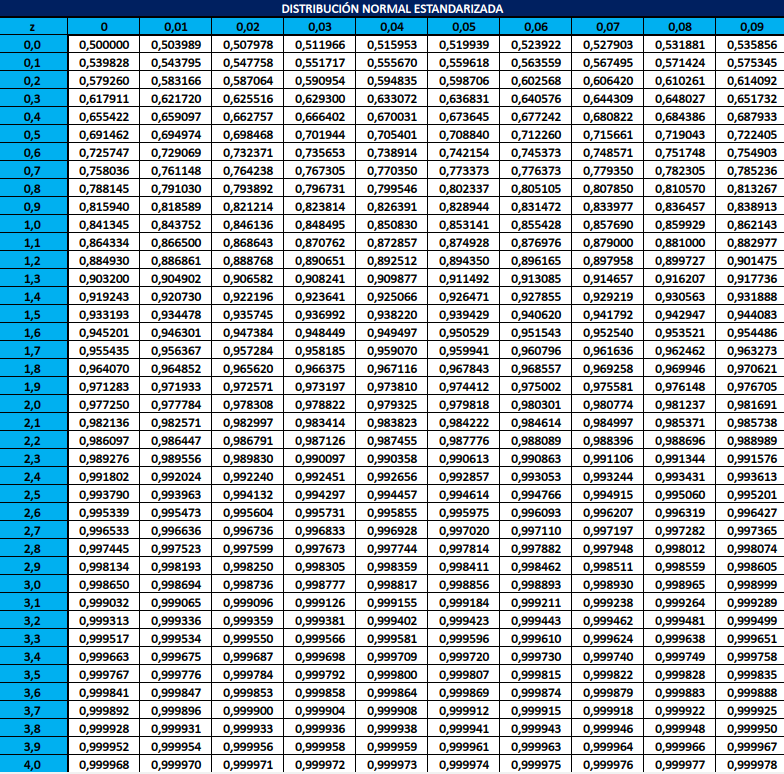
You can download this table in Excel format at the following link. I recommend reviewing that file because you will learn how to build your own table in case you cannot find one 🙂
How Do I Use This Table?
To use this table easily you must remember that, in addition to indicating a cumulative probability, it represents an area under the curve (of the density function). This can be seen represented in the following figure:
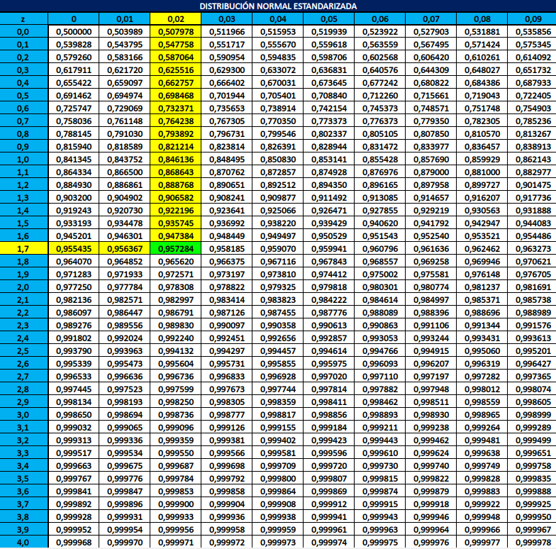
Having understood this, the next step is to explain the actual use of the table. What we see here is that the value z at which we will evaluate the function \Phi_{0,1}(z) is separated into two parts: in the column, you will find its expansion up to the first decimal digit, and in the row, you will find the second decimal digit; so, for example: the number z=1.72 can be found as if it were formed by “coordinates”: the vertical is 1.7, and the horizontal 0.02. Finally, the numerical approximation of \Phi_{0,1}(1.72) will appear in the block of coordinates “1.7” and “0.02”, which shows a value of 0.957284.
Exercises
- Estimate the value of \Phi_{0,1}(2.93)
- Estimate the value of \Phi_{\mu=12,\sigma=3}(11.5)
- A random variable X follows a normal distribution N(\mu=37,\sigma=9). Calculate P(35 \lt X \lt 43).
- The number of tomatoes that rot daily at a vendor’s stall has a mean \mu=50 with a standard deviation \sigma=15. If the vendor brings tomatoes 3 times a week, estimate the number of days in a month when more than 60 tomatoes will rot.
- Assuming that X \sim N(\mu,\sigma) calculate the following probabilities:
- P(\mu - \sigma \leq X \leq \mu + \sigma)
- P(X \leq \mu - \sigma \vee \mu + \sigma \leq X)
- P(X \leq \mu - n\sigma \vee \mu + n\sigma \leq X)