
実変数関数の極限
要約:
この授業では、実変数関数の極限の形式的定義を深く検討し、この定義に基づいて極限の代数則に至る主要な性質を証明します。
学習目標:
本授業の終了時に学生は次のことができるようになります:
- 実変数関数の極限の定義を想起する。
- \epsilon-\deltaの推論を用いて、極限の代数に至る性質を証明する。
- 極限の代数則およびその性質を用いて、実変数関数の極限を計算する。
目次
導入
関数の極限に関する直感的概念(グラフ的アプローチ)
極限の形式的定義
極限の性質
極限が存在するならば、それは一意である
極限の代数
基本的な極限の計算
導入
代数学と幾何学の学習と、解析学(微積分)の学習との違いは何か? この問いへの答えは、「極限」という概念によって明らかになります。本記事ではこのため、極限とその定義について学びます。
「極限」という語は、通常ある種の境界を連想させます。例えば区間 [a, b] の端点にある境界(その性質にかかわらず)などです。
[a,b[\;\; ;\;\; ]a,b]\;\; ; \;\; ]a,b[\;\; ; [a,b] ,
または、過去と未来の境界としての現在のように捉えることもできます。これと同様に、極限という概念は、ある点に漸近的に近づくという直感的なアイデアに対する数学的理解を導入するものです。
関数の極限に関する直感的概念(グラフ的アプローチ)
極限という概念を視覚的に捉えるために、まずは関数のグラフ表示から始めるのが適切です。そして、x が x_0 にどれほど近づくかに応じて f(x) がどうなるかを問うことになります。
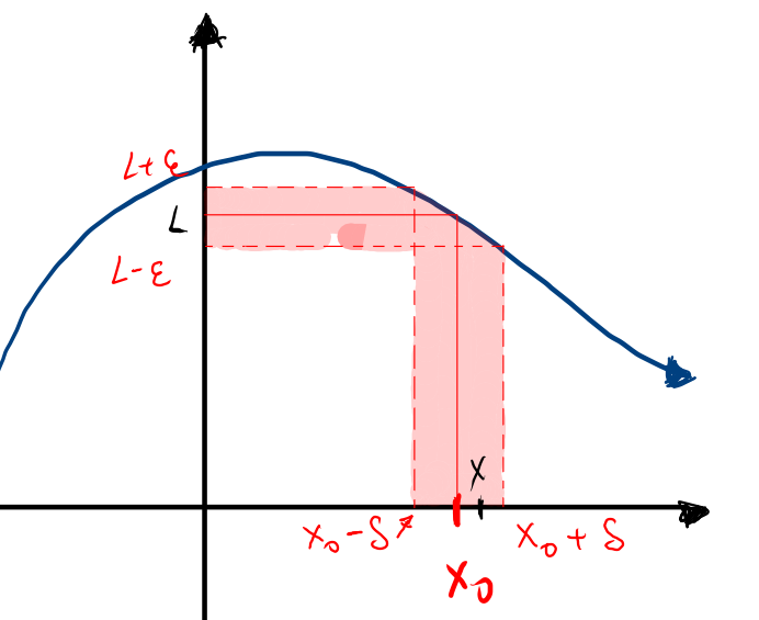
もし x が x_0 の近くにあるならば、中心が x_0 で半径が \delta の開区間が存在し、その中に x が含まれます。これは次の3つの形式で表すことができます:
|x-x_0|\lt \delta,
x\in]x_0 - \delta , x_0 + \delta[ ,
または x\in\mathcal{B}(x_0,\delta)
この文脈において、これらは同じ内容を示す3つの異なる表現です。ただし、最後の表現「中心 x_0、半径 \delta の開球体に含まれる x」という読み方は、より適切に位相空間論の講義などで、近傍の性質についてより深く掘り下げる場合に用いられます。
このような条件が成立するならば、中心 l、半径 \epsilon の開区間が存在し、その中に f(x) が含まれることになります。すなわち:|f(x) - l|\lt \epsilon。
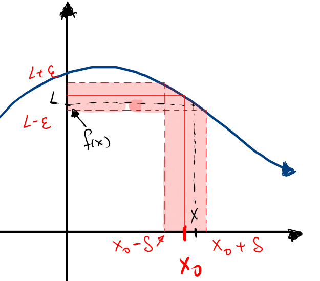
ここから、極限という数学的概念の基礎的な考え方が導かれます。それは、0 \lt|x-x_0|\lt \delta ならば |f(x)-l|\lt \epsilon が成り立つときに極限が存在し、このときの l が、x が x_0 に任意に近づくときの関数の極限値となります。
極限の形式的定義
先に述べた直感的かつ図的な考察から、形式的な極限の定義を明確にすることが可能になります。 極限が存在すると言うのは、\epsilon(つまり f(x) と l の距離)がどんなに小さくても、それに対応する \delta が常に存在して、0 \lt|x-x_0|\lt \delta のとき、|f(x) - l|\lt \epsilon が成り立つということです。この考え方は、初学者にとっては理解が難しく、世界中の多くの解析学の学生を泣かせる原因となっていますが、以下のような論理式で要約されます:
\displaystyle \lim_{x\to x_0}f(x)=l := \left(\forall \epsilon \gt 0\right)\left(\exists \delta\gt 0\right) \left(0 \lt|x-x_0|\lt\delta \rightarrow |f(x) - l|\lt \epsilon\right),
極限の性質
極限の形式的定義を持つことの意義は、それに基づいて極限の性質を証明できる点にあります。その中には直感的に明らかなものもあれば、そうでないものも含まれます。
これからの内容を理解しやすくするために、必須ではありませんが、数学的論理学のいくつかの基本概念を復習することを強く推奨します。
極限が存在するならば、それは一意である
この性質を証明するために、背理法(反証法)を用います。 まず、次の前提集合を定義することから始めます:
\displaystyle\mathcal{H}= \{\lim_{x\to x_0}f(x) = L, \lim_{x\to x_0}f(x) = L^\prime, L\neq L^\prime\}.
これをもとに、次のような形式的な証明を構築することができます:
| (1) | \displaystyle \mathcal{H}\vdash \lim_{x\to x_0}f(x) = L ;仮定 |
| \displaystyle \mathcal{H}\vdash \left(\forall \epsilon \gt 0\right)\left(\exists \delta\gt 0\right) \left(0 \lt|x-x_0|\lt\delta \rightarrow |f(x) - L|\lt \epsilon\right) | |
| (2) | \displaystyle \mathcal{H}\vdash \lim_{x\to x_0}f(x) = L^\prime ;仮定 |
| \displaystyle \mathcal{H}\vdash \left(\forall \epsilon \gt 0\right)\left(\exists \delta\gt 0\right) \left(0 \lt|x-x_0|\lt\delta \rightarrow |f(x) - L^\prime |\lt \epsilon\right) | |
| (3) | \displaystyle \mathcal{H}\vdash L \neq L^\prime ;仮定 |
| (4) | \displaystyle \mathcal{H}\vdash \left(\forall \epsilon \gt 0\right)\left(\exists \delta\gt 0\right) \left(0 \lt|x-x_0|\lt\delta \rightarrow\right. \left. \left[ \left( |f(x) - L |\lt \epsilon \right) \wedge \left( |f(x) - L^\prime |\lt \epsilon\right) \right] \right. );\wedge–導入(1,2) |
| (5) | \displaystyle \mathcal{H}\cup\{L\lt L^\prime\}\vdash \left(\forall \epsilon \gt 0\right)\left(\exists \delta\gt 0\right) \left(0 \lt|x-x_0|\lt\delta \rightarrow\right. \left. \left[ \left( |f(x) - L |\lt \epsilon \right) \wedge \left( |f(x) - L^\prime |\lt \epsilon\right) \right] \right. );単調性(4) |
| (6) | \displaystyle \mathcal{H}\cup\{L\lt L^\prime\}\vdash \epsilon = \frac{L - L^\prime}{2}\gt 0 ;なぜなら L \lt L^\prime だから |
| (7) | \displaystyle \mathcal{H}\cup\{L\lt L^\prime\}\vdash \left(\exists \delta\gt 0\right) \left(0 \lt|x-x_0|\lt\delta \rightarrow\right. \left. \left[ \left( |f(x) - L |\lt \frac{L - L^\prime}{2} \right) \wedge \left( |f(x) - L^\prime |\lt \frac{L - L^\prime}{2}\right) \right] \right. );(5,6) を使用 |
| \displaystyle \mathcal{H}\cup\{L\lt L^\prime\}\vdash (\exists \delta\gt 0) (0 \lt|x-x_0|\lt\delta \rightarrow [ ( 2 |f(x) - L |\lt L - L^\prime ) \wedge ( 2|f(x) - L^\prime |\lt L - L^\prime) ]) | |
| \displaystyle \mathcal{H}\cup\{L\lt L^\prime\}\vdash (\exists \delta\gt 0) (0 \lt|x-x_0|\lt\delta \rightarrow [ ( -L + L^\prime \lt 2 (f(x) - L )\lt L - L^\prime ) \wedge ( -L + L^\prime \lt 2(f(x) - L^\prime )\lt L - L^\prime) ]) | |
| \displaystyle \mathcal{H}\cup\{L\lt L^\prime\}\vdash (\exists \delta\gt 0) (0 \lt|x-x_0|\lt\delta \rightarrow [ ( -L + L^\prime \lt 2f(x) - 2L \lt L - L^\prime ) \wedge ( -L + L^\prime \lt 2f(x) - 2L^\prime \lt L - L^\prime) ]) | |
| \displaystyle \mathcal{H}\cup\{L\lt L^\prime\}\vdash (\exists \delta\gt 0) (0 \lt|x-x_0|\lt\delta \rightarrow [ ( L + L^\prime \lt 2f(x) \lt 3L - L^\prime ) \wedge ( -L + 3L^\prime \lt 2f(x) \lt L + L^\prime) ]) | |
| \displaystyle \mathcal{H}\cup\{L\lt L^\prime\}\vdash (\exists \delta\gt 0) (0 \lt|x-x_0|\lt\delta \rightarrow [ ( -L + 3L^\prime \lt 2f(x) \lt L + L^\prime) \wedge ( L + L^\prime \lt 2f(x) \lt 3L - L^\prime ) ]) | |
| (8) | \displaystyle \mathcal{H}\cup\{L\lt L^\prime\}\vdash \bot ;(1,2,6,7) より |
| (9) | \displaystyle \mathcal{H}\cup\{L\gt L^\prime\}\vdash \bot ;(8) と同様の手順 |
| (10) | \displaystyle \mathcal{H}\vdash [(L\lt L^\prime) \vee (L\gt L^\prime)] \rightarrow \bot ;\vee-導入(8,9) |
| (11) | \displaystyle \mathcal{H}\vdash [L\ \neq L^\prime] \rightarrow \bot ;定義(10) |
| (12) | \displaystyle \mathcal{H}\vdash \bot ;モーダスポネンス(3,11) |
| \displaystyle \left\{\lim_{x\to x_0}f(x) = L, \lim_{x\to x_0}f(x) = L^\prime, L\neq L^\prime\right\} \vdash \bot | |
| (13) | \displaystyle \left\{\lim_{x\to x_0}f(x) = L, \lim_{x\to x_0}f(x) = L^\prime \right\} \vdash \neg(L\neq L^\prime) ;背理法(12) |
| \displaystyle \left\{\lim_{x\to x_0}f(x) = L, \lim_{x\to x_0}f(x) = L^\prime \right\} \vdash L = L^\prime. |
この証明から、もし極限が2つ存在するならば、それらは等しく、したがって極限は一意であることがわかります。
極限の代数
これまでに、極限という数学的概念の基本を確認しました。 しかし、これだけでは極限の計算を行うには到底不十分です。極限の定義を直接用いて計算するのは、苦痛を求める狂人の所業と言えるでしょう。この問題を解決するために、ここからは極限を実際に計算するためのテクニックを学びます。
ここで、x_0, \alpha, \beta, L, M \in \mathbb{R}, とし、f と g を実関数で、次の関係を満たすとします:
\displaystyle \lim_{x\to x_0} f(x) = L
\displaystyle \lim_{x\to x_0} g(x) = M
このとき、次の性質が成り立ちます:
関数の和および差の極限
\displaystyle \lim_{x\to x_0} \left(\alpha f(x) \pm \beta g(x) \right) = \alpha L \pm \beta M
証明:
次の前提集合を考えましょう: \displaystyle\mathcal{H}=\left\{\lim_{x\to x_0} f(x) = L, \lim_{x\to x_0} g(x) = M \right\}。この集合から、次のような推論が可能です:
| (1) | \displaystyle \mathcal{H}\vdash \lim_{x\to x_0}f(x) = L ;仮定 |
| \displaystyle \mathcal{H}\vdash \left(\forall \epsilon \gt 0 \right)\left(\exists \delta \gt 0 \right) \left(0 \lt |x-x_0|\lt \delta \rightarrow |f(x) - L|\lt \epsilon \right) | |
| \displaystyle \mathcal{H}\vdash \left(\forall \epsilon \gt 0 \right)\left(\exists \delta \gt 0 \right) \left(0 \lt |x-x_0|\lt \delta \rightarrow |\alpha||f(x) - L|\lt |\alpha|\epsilon \right) | |
| \displaystyle \mathcal{H}\vdash \left(\forall \epsilon \gt 0 \right)\left(\exists \delta \gt 0 \right) \left( 0 \lt|x-x_0|\lt \delta \rightarrow |\alpha f(x) - \alpha L|\lt |\alpha|\epsilon \right) | |
| (2) | \displaystyle \mathcal{H}\vdash \overline{\epsilon}:= |\alpha|\epsilon ;定義 |
| (3) | \displaystyle \mathcal{H}\vdash \left(\forall \overline{\epsilon} \gt 0 \right)\left(\exists \delta \gt 0 \right) \left(0 \lt |x-x_0|\lt \delta \rightarrow |\alpha f(x) - \alpha L|\lt \overline{\epsilon} \right) ;(1,2) より |
| \displaystyle \mathcal{H}\vdash \lim_{x\to x_0}\alpha f(x) = \alpha L | |
| (4) | \displaystyle \mathcal{H}\vdash \lim_{x\to x_0}g(x) = M ;仮定 |
| (5) | \displaystyle \mathcal{H}\vdash \lim_{x\to x_0}\beta g(x) = \beta M ;(3) に類似 |
| \displaystyle \mathcal{H}\vdash \left(\forall \overline{\overline{\epsilon}} \gt 0 \right)\left(\exists \delta \gt 0 \right) \left( 0 \lt |x-x_0|\lt \delta \rightarrow |\beta g(x) - \beta M|\lt \overline{\overline{\epsilon}} \right) | |
| (6) | \displaystyle \mathcal{H}\vdash \left(\forall \overline{\epsilon},\overline{\overline{\epsilon}} \gt 0 \right)\left(\exists \delta \gt 0 \right) \left(0 \lt |x-x_0|\lt \delta \rightarrow \left[|\alpha f(x) - \alpha L|+ |\beta g(x) - \beta M|\lt \overline{\epsilon}+ \overline{\overline{\epsilon}} \right] \right) ;(3) と (5) より |
| (7) | \displaystyle \mathcal{H}\vdash |\alpha f(x) - \alpha L + \beta g(x) - \beta M| \leq |\alpha f(x) - \alpha L|+ |\beta g(x) - \beta M| ;三角不等式:(\forall x,y\in\mathbb{R})(|x+y|\leq |x|+|y|) |
| (8) | \displaystyle \mathcal{H}\vdash \left(\forall \overline{\epsilon},\overline{\overline{\epsilon}} \gt 0 \right)\left(\exists \delta \gt 0 \right) \left(0 \lt |x-x_0|\lt \delta \rightarrow |\alpha f(x) - \alpha L + \beta g(x) - \beta M| \lt \overline{\epsilon}+ \overline{\overline{\epsilon}} \right) ;(6,7) より |
| (9) | \epsilon^* := \overline{\epsilon} + \overline{\overline{\epsilon}};定義 |
| (10) | \displaystyle \mathcal{H}\vdash \left(\forall \epsilon^* \gt 0 \right)\left(\exists \delta \gt 0 \right) \left(0 \lt |x-x_0|\lt \delta \rightarrow |\alpha f(x) + \beta g(x) - \alpha L - \beta M| \lt \epsilon^* \right) ;(8,9) より |
| \displaystyle \mathcal{H}\vdash \lim_{x\to x_0} (\alpha f(x) + \beta g(x)) = \alpha L + \beta M | |
| (11) | \gamma:= - \beta;定義 |
| (12) | \displaystyle \mathcal{H}\vdash \lim_{x\to x_0} (\alpha f(x) + \gamma g(x)) = \alpha L + \gamma M ;(10) に類似 |
| (13) | \displaystyle \mathcal{H}\vdash \lim_{x\to x_0} (\alpha f(x) - \beta g(x)) = \alpha L - \beta M ;(11,12) より |
| (14) | \displaystyle \mathcal{H}\vdash \lim_{x\to x_0} (\alpha f(x) \pm \beta g(x)) = \alpha L \pm \beta M ;(10,13) より |
関数の積の極限
\displaystyle \lim_{x\to x_0} \left( f(x) g(x) \right) = L M
この証明は前のものより少し難しいですが、 いくつかのドラコニアンなテクニックを使えば十分解決可能です。前の証明と同じ前提集合 \mathcal{H} を用いて、次のような推論を構築することができます:
| (1) | \displaystyle \mathcal{H}\vdash \overline{\epsilon} := \frac{|\epsilon|}{2(|M|+1)} \leq \frac{|\epsilon|}{2} ;定義 |
| (2) | \displaystyle \mathcal{H}\vdash \lim_{x\to x_0} f(x) = L ;仮定 |
| \displaystyle \mathcal{H}\vdash \left(\forall \overline{\epsilon} \gt 0 \right)\left(\exists \delta \gt 0 \right)\left(0 \lt |x-x_0|\lt \delta \rightarrow |f(x) - L| \lt \overline{\epsilon} = \frac{|\epsilon|}{2(|M|+1)}\right) ;(1) を使用 | |
| (3) | \displaystyle \mathcal{H}\vdash \overline{\overline{\epsilon}} := \frac{|\epsilon|}{2(|L|+1)} \leq \frac{|\epsilon|}{2};定義 |
| (4) | \displaystyle \mathcal{H}\vdash \lim_{x\to x_0} g(x) = M ;仮定 |
| \displaystyle \mathcal{H}\vdash \left(\forall \overline{\overline{\epsilon}} \gt 0 \right)\left(\exists \delta \gt 0 \right)\left(0 \lt |x-x_0|\lt \delta \rightarrow |g(x) - M| \lt \overline{\overline{\epsilon}} = \frac{|\epsilon|}{2(|L|+1)}\right) ;(3) を使用 | |
| (5) | \displaystyle \mathcal{H}\vdash |f(x)| - |L| \lt |f(x) - L| \lt \overline{\epsilon} \lt 1 ;三角不等式+\overline{\epsilon} の特別な場合 |
| (6) | \displaystyle \mathcal{H}\vdash |f(x)|\lt 1 + |L| ;(5) より |
| (7) | \displaystyle \mathcal{H}\vdash |g(x)| - |M| \lt |g(x) - M| \lt \overline{\overline{\epsilon}} \lt 1 ;三角不等式+\overline{\overline{\epsilon}} の特別な場合 |
| (8) | \displaystyle \mathcal{H}\vdash |g(x)| \lt 1 + |M| ;(7) より |
| (9) | \displaystyle \mathcal{H}\vdash |f(x)g(x) - LM|=| f(x)g(x) - Mf(x) + Mf(x) - LM |;ゼロの加算 |
| \displaystyle \mathcal{H}\vdash |f(x)g(x) - LM|=| f(x)(g(x) - M) + M (f(x) - L) |;因数分解 | |
| (10) | \displaystyle \mathcal{H}\vdash |f(x)g(x) - LM|\leq | f(x)(g(x) - M) | + | M (f(x) - L) |;三角不等式より (9) |
| \displaystyle \mathcal{H}\vdash |f(x)g(x) - LM|\leq |f(x)||g(x) - M| + |M| |f(x) - L| | |
| (11) | \displaystyle \mathcal{H}\vdash |f(x)g(x) - LM|\lt (1 + |L|)|g(x) - M| + |M|\overline{\epsilon};(5,6,10) より |
| (12) | \displaystyle \mathcal{H}\vdash \left[ |g(x) - M|\lt \overline{\overline{\epsilon}} \right] \rightarrow \left[ (1+|L|)|g(x) - M| + |M|\overline{\epsilon} \lt (1+|L|)\overline{\overline{\epsilon}} + |M|\overline{\epsilon}\right];(11) より |
| (13) | \displaystyle \mathcal{H}\vdash \left[ |g(x) - M|\lt \overline{\overline{\epsilon}} \right] \rightarrow \left[ (1+|L|)|g(x) - M| + |M|\overline{\epsilon} \lt (1+|L|)\frac{|\epsilon|}{2(|L|+1)} + |M|\frac{|\epsilon|}{2(|M|+1)}\right];(1,3,12) より |
| \displaystyle \mathcal{H}\vdash \left[ |g(x) - M|\lt \overline{\overline{\epsilon}} \right] \rightarrow \left[ (1+|L|)|g(x) - M| + |M|\overline{\epsilon} \lt \frac{|\epsilon|}{2} + \frac{|\epsilon||M|}{2(|M|+1)} \lt \frac{|\epsilon|}{2}+ \frac{|\epsilon|}{2} = |\epsilon| \right] | |
| (14) | \displaystyle \mathcal{H}\vdash \left[ |g(x) - M|\lt \overline{\overline{\epsilon}} \right] \rightarrow \left[ |f(x)g(x) - LM|\lt |\epsilon| \right];(11,13) より |
| (15) | \displaystyle \mathcal{H}\vdash (\forall \epsilon \gt 0 ) (\exists \delta \gt 0 ) \left(0 \lt |x-x_0|\lt \delta \rightarrow |f(x)g(x) - LM|\lt |\epsilon| \leq \epsilon \right) ;(1,2,4,14) より |
| \displaystyle \mathcal{H}\vdash \lim_{x\to x_0}f(x)g(x) = LM. |
定数関数の極限
定数関数 f(x)=c の極限は、定数 c そのものです。すなわち、
\displaystyle \lim_{x\to x_0}c = c
証明
この証明は実に簡単で、実際にはトートロジー(恒真命題)です。すでに以下が知られています:
\displaystyle \lim_{x\to x_0}c = c := (\forall\epsilon\gt 0) (\exists \delta \gt 0)(0\lt|x-x_0|\lt \delta \rightarrow |c-c|\lt \epsilon)
しかし、0=|c-c|\lt \epsilon は任意の正の ε に対して常に成り立つため、含意全体もまたトートロジーとなり、したがって表現 \displaystyle \lim_{x\to x_0}c = c もトートロジーです。
関数の商の極限
次に、2つの関数の商の極限に関する法則を証明する準備が整いました。 それは次の通りです:
\displaystyle \lim_{x\to x_0}\frac{f(x)}{g(x)}= \frac{L}{M}
ここでも、前の性質と同様に、次の前提集合が成立しているものとします:
\displaystyle \mathcal{H}=\{\lim_{x\to x_0}f(x) = L, \lim_{x\to x_0}g(x) = M\}
証明
幸いにも、これまでのような証明を繰り返す必要はありません。すでに得られた結果を用いて目的を達成できるからです。ただしその前に、次の関係をまず証明しましょう:
\displaystyle \lim_{x\to x_0}\frac{1}{g(x)} = \frac{1}{M}
これを証明するには、積の極限の法則と定数関数の極限を組み合わせて用いれば十分です。ただし、g(x) が 0 でないことに注意しなければなりません:
\displaystyle 1 = \lim_{x\to x_0}\left( 1 \right) \lim_{x\to x_0}\left( g(x) \cdot \frac{1}{g(x)} \right) = \lim_{x\to x_0}g(x) \cdot \lim_{x\to x_0} \frac{1}{g(x)} = M \cdot \lim_{x\to x_0} \frac{1}{g(x)}
したがって:\displaystyle \lim_{x\to x_0} \frac{1}{g(x)} = \frac{1}{M}
最後に、積の極限の法則より次のようになります:
\displaystyle \lim_{x\to x_0} \frac{f(x)}{g(x)} = \lim_{x\to x_0} f(x) \frac{1}{g(x)}= L \cdot\frac{1}{M} = \frac{L}{M}
これは M が 0 でない限り常に成り立ちます。
自然数乗の極限
この性質は次のように述べられます。 もし \displaystyle \lim_{x_0 \to x_0}f(x) = L であるならば、\displaystyle \left(\forall n \in \mathbb{N}\right) \left( \lim_{x\to x_0} \left( [f(x)]^n \right) = L^n \right) が成り立ちます。これは数学的帰納法により証明できます。
証明:
- 場合 n=1:(初期ステップ)
\displaystyle \lim_{x\to x_0} [f(x)]^1 = \lim_{x\to x_0} f(x) = L. これは初期ステップの完了を意味します ✅
- 場合 n=k:(帰納ステップ)
仮定として:\displaystyle \lim_{x\to x_0} [f(x)]^k = L^k が成り立つとすると(帰納法の仮定)、次が成り立つことを示します:\displaystyle \lim_{x\to x_0} [f(x)]^{k+1} = L^{k+1}
次のように分解できます:\displaystyle \lim_{x\to x_0} [f(x)]^{k+1} = \lim_{x\to x_0} \{f(x) [f(x)]^k\} = \lim_{x\to x_0}f(x) \lim_{x\to x_0} [f(x)]^{k} =L \lim_{x\to x_0} [f(x)]^{k}。これは上で証明された積の極限の法則によります。
したがって、帰納仮定により \displaystyle \lim_{x\to x_0} [f(x)]^{k+1} = L \lim_{x\to x_0} [f(x)]^{k} =L\cdot L^k = L^{k+1}. 帰納ステップも完了 ✅
- よって:\displaystyle \left(\forall n \in \mathbb{N}\right) \left( \lim_{x\to x_0} \left( [f(x)]^n \right) = L^n \right).
n乗根の極限
乗の極限と同様に、次が成り立ちます。 \displaystyle \left(\forall n \in \mathbb{N}\right) \left( \lim_{x\to x_0} \sqrt[n]{f(x)} = \sqrt[n]{L} \right)
証明:
先ほど証明したべき乗の極限の性質を用いて:
\displaystyle L= \lim_{x\to x_0} f(x)=\lim_{x\to x_0} \left[\sqrt[n]{f(x)}\right]^n = \left[ \lim_{x\to x_0} \sqrt[n]{f(x)}\right]^n
したがって:\displaystyle \lim_{x\to x_0} \sqrt[n]{f(x)} =\sqrt[n]{L}.
分数べきの極限
これまでの2つの性質を組み合わせることで、 最後の証明として次を導くことができます: \displaystyle \left(\forall p,q\neq 0 \in \mathbb{Z}\right) \left( \lim_{x\to x_0} \left[f(x)\right]^{\frac{p}{q}} = L^{\frac{p}{q}} \right).
これは積の極限の法則によって、次のように変形されるためです:
\displaystyle [f(x)]^{\frac{p}{q}} =[\sqrt[q]{f(x)}]^p 、\displaystyle L^{\frac{p}{q}} =[\sqrt[q]{L}]^p.
極限 \displaystyle \lim_{x\to x_0}x = x_0
この証明によって、これまでの一連の証明を締めくくります。これらの結果を活用することで、今後は多くの極限をほぼ直感的に計算できるようになります。
\displaystyle \lim_{x\to x_0}x = x_0 を証明するのは簡単です。これが成立するためには、次の条件が必要です:
(\forall \epsilon \gt 0) (\exists \delta \gt 0)(0\lt |x-x_0|\lt \delta\rightarrow |x-x_0|\lt \epsilon)
極限の定義によれば、任意のイプシロンに対して、あるデルタが存在し、その他の条件がすべて成り立つ必要があります。したがって、少なくとも1つのデルタが見つかれば十分です。実際にはこれは自明であり、任意の \delta\leq\epsilon をとればこの条件を満たします。よって:\displaystyle \lim_{x\to x_0}x = x_0.
基本的な極限の計算
これまで確認してきたすべての定理を用いれば、多くの極限を関数に単に代入するような感覚で、非常に直感的に計算できます。以下にいくつかの例を示します:
- {}\\ \begin{array}{rl} \displaystyle \lim_{x\to 2}(x^2 + 4x) & = \displaystyle \lim_{x\to 2}(x^2) + \lim_{x\to 2}(4x) \\ \\ & = \displaystyle \left(\lim_{x\to 2} x \right)^2 + 4\lim_{x\to 2} x \\ \\ & = (2)^2 + 8 = 12 \end{array}
- {} \\ \begin{array}{rl} \displaystyle \lim_{x\to 1}\left.\frac{(3x-1)^2}{(x+1)^3} \right. & = \displaystyle \frac{(3(1)-1)^2}{((1)+1)^3} \\ \\ & = \displaystyle \frac{4}{8} = \frac{1}{2} \end{array}
- {} \\ \begin{array}{rl} \displaystyle \lim_{x\to 2} \frac{x-2}{x^2 - 4} &= \displaystyle \lim_{x\to 2} \frac{x-2}{(x-2)(x+2)} \\ \\ & = \displaystyle \lim_{x\to 2} \frac{1}{x+2} = \dfrac{1}{4} \end{array}
- {} \\ \begin{array}{rl} \displaystyle \lim_{h\to 0} \frac{(x+h)^3-x^3}{h} &= \displaystyle \lim_{h\to 0} \frac{x^3 + 3x^2 h + 3xh^2 -x^3}{h} \\ \\ & = \displaystyle\lim_{h\to 0} \frac{3x^2 h + 3xh^2}{h} \\ \\ & = \displaystyle \lim_{h\to 0} 3x^2 + 3xh = 3x^2 \end{array}
- {} \\ \begin{array}{rl} \displaystyle \lim_{x\to 1} \frac{x-1}{\sqrt{x^2 + 3} - 2 } &=\displaystyle \lim_{x\to 1} \frac{x-1}{\sqrt{x^2 + 3} - 2 } \frac{\sqrt{x^2 + 3} + 2}{\sqrt{x^2 + 3} + 2} \\ \\ & =\displaystyle \lim_{x\to 1} \frac{(x-1)(\sqrt{x^2 + 3} + 2)}{(x^2 + 3) - 4 } \\ \\ & =\displaystyle \lim_{x\to 1} \frac{(x-1)(\sqrt{x^2 + 3} + 2)}{x^2 -1 } \\ \\ & =\displaystyle \lim_{x\to 1} \frac{(x-1)(\sqrt{x^2 + 3} + 2)}{(x-1)(x+1) } \\ \\ & =\displaystyle \lim_{x\to 1} \frac{\sqrt{x^2 + 3} + 2}{ x+1 } \\ \\ & =\displaystyle \frac{2+2}{2} =2 \end{array}