Introduction

We have already studied how refraction works; that is, what happens when light passes from one medium to another. But we have done all this assuming that the interface separating the media is a flat surface. However, both in nature and in practical applications, it is not difficult to find refraction processes at spherical interfaces. Examples of these include the human eye (and almost any animal eye, actually) and most optical devices used in everyday life and industrial applications.

In the following figure, we see how a lens is constructed through two spherical surfaces.

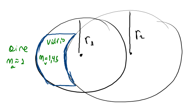
For a detailed study of this type of device, it is necessary to review how light behaves when passing from one medium to another through a spherical interface.

The Object-Image Relationship for Refraction at Spherical Interfaces

We will begin our study by investigating how light behaves when passing from one medium to another through a spherical interface. To do this, we will consider a sphere of radius R made of a material with a refractive index n_b immersed in a medium with a refractive index n_a.

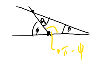
Extracting Relationships Between Angles

If we analyze the angles involved in this figure, we will notice that:

\begin{array}{rll} {(1)}& \theta_a & =\alpha + \phi \\ \\ {(2)}& \phi & =\beta + \theta_b \end{array}

Proof

The first equation is obtained from the fact that the sum of the interior angles of a triangle is equal to two right angles:

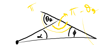
\begin{array}{rl} & \alpha + \phi + (\pi - \theta_a) = \pi\\ \\ \equiv & \alpha + \phi - \theta_a = 0 \\ \\ \equiv & \color{blue}{\theta_a = \alpha + \phi} \end{array}

The second is obtained in a similar manner:

\begin{array}{rl} & \beta + \theta_b + (\pi - \phi) = \pi\\ \\ \equiv & \beta + \theta_b - \phi = 0\\ \\ \equiv & \color{blue}{\phi = \beta + \theta_b } \end{array}

Introducing Snell’s Law

From the figure, we also have the following expressions:

\begin{array}{rll} {(3)}&\tan(\alpha) &=\displaystyle \frac{h}{s+\delta}\\ \\ {(4)}&\tan(\beta) &=\displaystyle \frac{h}{s^\prime - \delta}\\ \\ {(5)}&\tan(\phi) &=\displaystyle \frac{h}{R - \delta} \end{array}

And from Snell’s Law we have

\begin{array}{rl} {(6)} & n_a\sin(\theta_a) = n_b \sin(\theta_b)\end{array}

Now, if we take the approximation where \theta_a and \theta_b are small, then \alpha, \beta and \phi will also be small, and it will follow that:

From the figure, we also have the following expressions:

\begin{array}{rl} \sin(\theta_a) &\approx \theta_a \\ \\ \sin(\theta_b) &\approx \theta_b \\ \\ \delta &\approx 0 \\ \\ \tan(\alpha) &\approx \alpha \\ \\ \tan(\beta) &\approx \beta \\ \\ \tan(\phi) &\approx \phi \end{array}

Then, from this and Snell’s Law, we have:

\begin{array}{rl} {(7)} & n_a \theta_a \approx n_b \theta_b \\ \\ \equiv & \theta_b \approx \displaystyle \frac{n_a}{n_b} \theta_a \end{array}

Now, from (7), (1), and (2) we have

\begin{array}{rl} {(8)} & \phi - \beta \approx \displaystyle \frac{n_a}{n_b}(\alpha + \phi) \\ \\ \equiv & \phi \approx \beta + \displaystyle \frac{n_a}{n_b}(\alpha + \phi) \\ \\ {}\equiv & n_b\phi \approx n_b\beta + n_a \alpha + n_a\phi \\ \\ \equiv & \color{blue}{n_a \alpha + n_b\beta \approx (n_b - n_a) \phi } \end{array}

Finally, from (8), the approximations, and the equations (3), (4), and (5), we arrive at:

\begin{array}{rl} {(9)} & \displaystyle n_a \left( \frac{\color{red}{h}}{S + \underbrace{\delta}_{\to 0}} \right) + n_b \left(\frac{\color{red}{h}}{S^\prime - \underbrace{\delta}_{\to 0} } \right) \approx (n_b - n_a) \left(\frac{\color{red}{h}}{R-\underbrace{\delta}_{\to 0}}\right) \\ \\ \equiv & \displaystyle \color{blue}{\frac{n_a}{S } + \frac{ n_b}{S^\prime } \approx \frac{n_b - n_a}{R} } \end{array}

This last equation is what we call the Object-Image Relationship for Refraction at Spherical Interfaces.

Formation of Extended Images by Refraction on the Other Side of Spherical Interfaces

Now let’s see what happens when we change the point light source to an extended object. This is illustrated in the following figure:

The previous analysis already indicates the relationship between S and S^\prime, now we only need to find the relationship between the sizes of the object and the image.

From the figure, we have:

\begin{array}{rl} \tan(\theta_a) & =\displaystyle \frac{y}{S} \\ \\ \tan(\theta_b) & =\displaystyle - \frac{y^\prime}{S^\prime} \end{array}

We will combine this with Snell’s Law

n_a\sin(\theta_a) = n_b\sin(\theta_b).

And for this, we will rely on the fact that for small angles the approximation holds

\begin{array}{rl} \sin(\theta_a) & \approx \tan(\theta_a) \\ \\ \sin(\theta_b) & \approx \tan(\theta_b) \end{array}

So that we can write

\begin{array}{rl} &\displaystyle n_a \frac{y}{S} \approx- n_b \dfrac{y^\prime}{S^\prime} \\ \\ \equiv & \displaystyle \dfrac{y^\prime}{y} \approx - \dfrac{n_a S^\prime}{n_b S} \\ \\ \end{array}

Now, recalling what we have seen for spherical mirrors, we have something analogous. At this point, we can (re)define the magnification factor m as:

m=\displaystyle \frac{y^\prime}{y}

so that:

\displaystyle \color{blue}{m\approx -\frac{n_a S^\prime}{n_b S}}

Synthesis

In summary, so far we have extracted two results that allow us to infer the formation of images when light emitted from an object passes through a spherical interface. These are the following equations:

\begin{array}{rl} \displaystyle \dfrac{n_a}{S} + \dfrac{n_b}{S^\prime} & \approx \dfrac{n_b - n_a}{R} \\ \\ m & \displaystyle \approx - \dfrac{n_a S^\prime}{n_b S} \end{array}

With these two equations, you can calculate both the position of the image and the orientation and size of the image, and they will work regardless of whether the interface surface is concave or convex. At this point, however, it is necessary to clarify the sign convention.

Sign Convention

With these two equations, you can calculate both the position of the image and the orientation and size of the image, and they will work regardless of whether the interface surface is concave or convex. At this point, however, it is necessary to clarify the sign convention.

The interface divides the space into two regions, one where the object can be found and the other where the image is located. Based on this, we have:

• Object position S: Positive if it is on the object’s side, negative if it is on the image’s side.
• Image position S^\prime and radius of curvature R: Positive if it is on the image’s side, negative if it is on the object’s side.
• Object and image size, y and y^\prime: Positive if it is above the optical axis, negative if it is below the optical axis.

Flat Interfaces as a Limiting Case of Spherical Ones

Everything we have developed for spherical interfaces also helps to better understand flat interfaces. In fact, we can understand a flat interface as a piece of a spherical interface with a very large radius of curvature; indeed, if we take limits on the object-image relationship for spherical interfaces as the radius tends to infinity, we have:

\displaystyle \frac{n_a}{S } + \frac{ n_b}{S^\prime} = \lim_{R\to \infty} \frac{n_a}{S } + \frac{ n_b}{S^\prime } \approx \lim_{R\to \infty} \frac{n_b - n_a}{R} = 0

And if from this we calculate the magnification factor, we get:

m=1

That is, the image retains its size and orientation, what does vary is its observed position.

Exercises

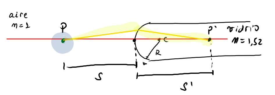
1. In front of a cylindrical glass rod, a particle is placed as shown belowIf the particle is 30[cm] from the rod and the tip of the rod is approximately spherical with a radius R=1.5[cm], calculate the position of the image generated inside the rod.
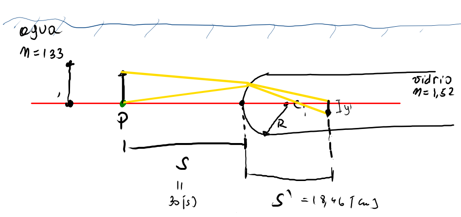
2. Let’s consider the same rod from the previous exercise, but now it is underwater. If a needle 1[cm] tall is placed in front of it at the same distance of 30[cm], calculate the location and height of the image.
3. A person looks into the bottom of a pool to estimate its depth. As a guide, they use an arrow painted on the bottom. What is the relationship between the real and apparent depth?