

The Squeeze Theorem for Calculating Limits
Summary:
This class presents the Squeeze Theorem, a key tool in calculus for evaluating difficult limits using simpler functions that bound from above and below. It offers a graphical explanation and a formal proof, followed by practical examples. The goal is for students to understand how to apply this theorem to calculate limits more efficiently.
Learning Objectives:
Upon completing this class, the student will be able to
- Understand the utility of the Squeeze Theorem in limit calculation.
- Identify functions that can bound a target function to apply the theorem.
- Apply the Squeeze Theorem to calculate difficult limits.
- Visualize the concept of the Squeeze Theorem graphically.
- Prove the Squeeze Theorem formally.
TABLE OF CONTENTS:
Introduction
Graphical Idea of the Squeeze Theorem
Proof of the Squeeze Theorem
Examples
Introduction
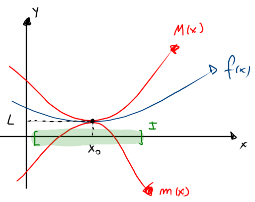
The utility of the Squeeze Theorem lies in its ease of calculating some difficult limits through simpler ones. The reason for the name is that, instead of directly calculating the limit of a function as x\to x_0, another pair of functions is used, one bounding from above and the other from below, whose limit at x_0 coincides and is easy to obtain. Since the original function is always between the two, it is like “the cheese between the two slices of bread.”
Graphical Idea of the Squeeze Theorem
The idea that synthesizes the theorem is actually quite simple. Let’s suppose we want to calculate a difficult limit
\displaystyle\lim_{x \to x_0}f(x)
What is usually done is to take all our knowledge of function algebra to try to simplify it to the point where we can evaluate it. However, sometimes a different approach is much more efficient. Suppose we have a closed interval I such that x_0 \in I and there also exist two other functions m(x) and M(x) that satisfy the relation
(\forall x\in I)(m(x)\leq f(x) \leq M(x) )
And also
\displaystyle \lim_{x\to x_0} m(x) = \lim_{x\to x_0} M(x) = L
Then it will follow that
\displaystyle \lim_{x\to x_0} f(x) = L
This is what we can see in the following image.
Proof of the Squeeze Theorem
To prove the Squeeze Theorem, we will follow the following reasoning:
| (1) | x_0\in I; Premise |
| (2) | \displaystyle \lim_{x\to x_0} m(x) = L ; Premise |
| (\forall \epsilon \gt 0)(\exists \delta_1 \gt 0) (|x-x_0|\lt \delta_1 \rightarrow |m(x) -L| \lt \epsilon ) | |
| (3) | \displaystyle \lim_{x\to x_0} M(x) = L ; Premise |
| (\forall \epsilon \gt 0)(\exists \delta_2 \gt 0) (|x-x_0|\lt \delta_2 \rightarrow |M(x) -L| \lt \epsilon ) | |
| (4) | (\forall x \in I)(m(x) \leq f(x) \leq M(x) ); Premise |
| (5) | (\forall x \in I)(m(x) - L \leq f(x) - L \leq M(x) - L ); From (4) |
| (6) | (|m(x) -L|\lt \epsilon) \rightarrow (-\epsilon \lt m(x) - L \lt \epsilon) |
| (7) | (|M(x) -L|\lt \epsilon ) \rightarrow (-\epsilon \lt M(x) - L \lt \epsilon) |
| (8) | (\forall \epsilon \gt 0)(\exists \delta \gt 0) (|x-x_0|\lt \delta=\min\{\delta_1,\delta_2\} \rightarrow ( |M(x) -L| \lt \epsilon \wedge |m(x) -L| \lt \epsilon ) ); From (2,3) |
| (9) | (\forall \epsilon \gt 0)(\exists \delta \gt 0) (|x-x_0|\lt \delta=\min\{\delta_1,\delta_2\} \rightarrow ( - \epsilon \lt f(x) - L \lt \epsilon ) ); From (1,5,6,7,8) |
| (\forall \epsilon \gt 0)(\exists \delta \gt 0) (|x-x_0|\lt \delta=\min\{\delta_1,\delta_2\} \rightarrow |f(x) - L| \lt \epsilon ) ) | |
| \displaystyle \lim_{x\to x_0}f(x) = L\;\blacksquare |
Examples
Using the Squeeze Theorem, we can calculate the limit of functions even when we don’t have their explicit algebraic expression. Here are a couple of examples:
An example of this occurs in the following situation:
- If \sqrt{5-2x^2}\leq f(x) \leq \sqrt{5-x^2}, when -1\leq x\leq 1. What is the value of \displaystyle \lim_{x\to 0}f(x)? [SOLUTION]
Another practical use of the Squeeze Theorem occurs when the limit itself is not evident compared to other simpler limits that bound it from above and below, such as what is obtained when calculating the following case:
- Calculate: \displaystyle \lim_{x\to 0}\dfrac{\sin(x)}{x} [SOLUTION]