LEARNING OBJECTIVES:
By the end of this class, students will be able to:

1. Recall the basic definitions of position, velocity, and acceleration in kinematics.
2. Analyze the relationships between acceleration, velocity, and position.
3. Apply derivatives and integrals to calculate velocity and position from acceleration, and vice versa.
4. Understand the difference between instantaneous and average velocity, and between instantaneous and average acceleration.

Introduction

From acceleration, it is possible to calculate velocity and position through integration with respect to time, and from position, we can calculate velocity and acceleration through differentiation with respect to time. These words summarize what we will explore about kinematics, and one of our main objectives will be to understand the meaning of these terms. Motion represents a form of change, and everything in nature is subject to change. Therefore, the study of change and its variations is one of the fundamental pillars of physics.

There are many variables susceptible to change: the new becomes old, one can change from one profession to another, from healthy to sick and vice versa, and from day to night, among others. All these are examples of changes, but when studying kinematics, we will focus on one in particular: the change in position or motion. In the study of motion, we can appreciate two complementary approaches: one based on the causes that produce it and another on the way it unfolds, giving rise to Dynamics and Kinematics, which together form Mechanics.

In physics, we model physical space as a vector space to facilitate the mathematical representation of concepts such as position, velocity, and acceleration. Commonly, we use the three-dimensional space \mathbb{R}^3 for this purpose, although in theory, spaces of any dimension can be suitable according to the context.

Position, Space, and Observers

Let’s consider a function

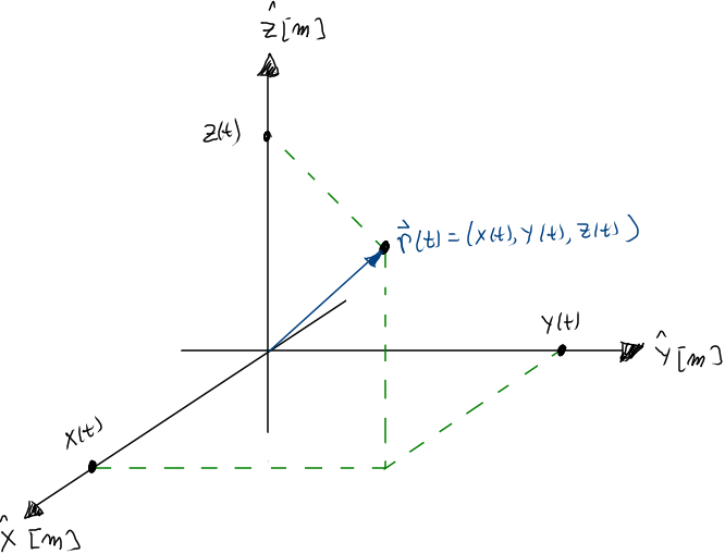
\begin{array}{rll} \vec{r}:\mathbb{R}[T]&\longrightarrow&\mathbb{R}^n[L] \\ t &\longmapsto&\vec{r}(t) \end{array}

This is a function that assigns a position \vec{r}(t) to each t\in\mathbb{R}, and thus, we say it is a position function (or simply position). The independent variable t is called “time,” and the parameter n corresponds to the “dimension” of the space. The symbols [T] and [L] refer to the physical dimensions of time and length, generally measured in “seconds” and “meters,” respectively.

Position, like any physical quantity, is measured by an observer. In the description I have given of the position, I have implicitly assumed that the observer has the coordinates of the null vector, \vec{0}. If the observer \mathcal{O} has the coordinates of the vector \vec{r} and the point object has coordinates \vec{r}^\prime, then the position relative to the observer will be:

\vec{r}_\mathcal{O} = \vec{r} - \vec{r}^\prime

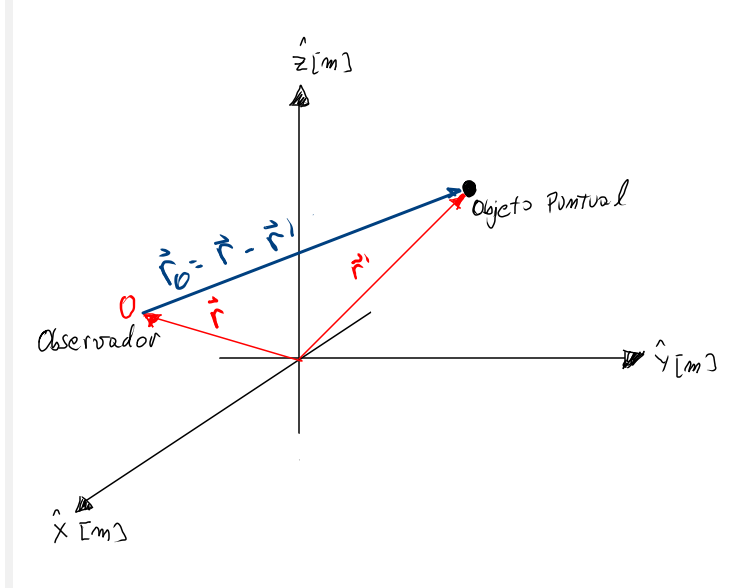
Space is the set of all possible positions, it is also the set of all possible positions relative to any observer. Position is a function of time and is used to mathematically represent the place where an ideal object called “point object” is found at each instant t. The point object is an idealization, it is what remains of a real object when we strip it of all its qualities, including size and shape, keeping only the “place it occupies in space.”

Position is generally a vector. Vectors are composed of two elements: magnitude and direction. The magnitude of the position relative to an observer is the distance to the observer and is given by dist_\mathcal{O}(t)=\|\vec{r}_\mathcal{O}(t)\|.

From this point, it is highly recommended to master the contents of the course on calculus differential and integral.

Speed and Velocity

If position is differentiable with respect to time, then it is possible to define the velocity relative to an observer \mathcal{O}, \vec{v}_\mathcal{O}(t), as follows:

\vec{v}_\mathcal{O}(t) =\displaystyle \lim_{\Delta t \to 0}\frac{\vec{r}_\mathcal{O}(t+\Delta t) - \vec{r}_\mathcal{O}(t)}{\Delta t} = \frac{d\vec{r}_\mathcal{O}(t)}{dt}

In simple terms: velocity is the temporal derivative of position and tells us how the position changes at each moment t.

There are two types of velocities: instantaneous and average. The instantaneous velocity is the one just presented, the average velocity is obtained by omitting the limit calculation. The average velocity over the time interval of length \Delta t, \left< \vec{v}_{\mathcal{O},\Delta t}(\overline{t}) \right>, is defined as

\left< \vec{v}_{\mathcal{O},\Delta t}(\overline{t}) \right> = \displaystyle \frac{\vec{r}_\mathcal{O}(t+\Delta t) - \vec{r}_\mathcal{O}(t)}{\Delta t}

where \overline{t} is any moment contained in the interval [t,t+\Delta t].

From the velocity (whether instantaneous or average) speed is defined as its corresponding magnitude. The speed relative to an observer \mathcal{O} is v_\mathcal{O}(t)=\|\vec{v}_\mathcal{O}(t)\|, and the average speed \left< {v}_{\mathcal{O},\Delta t}(\overline{t}) \right> = \|\left< \vec{v}_{\mathcal{O},\Delta t}(\overline{t}) \right>\|.

Speed and velocity are measured in units of length over units of time, [L/T], generally in “meters per second”.

Acceleration

Similarly to velocity, if it is differentiable with respect to time, then it is possible to define the concept of acceleration relative to an observer \mathcal{O}, \vec{a}_\mathcal{O}(t), as follows:

\vec{a}_\mathcal{O}(t)= \displaystyle \lim_{\Delta t \to 0}\frac{\vec{v}_\mathcal{O}(t+\Delta t) - \vec{v}_\mathcal{O}(t)}{\Delta t} = \frac{d\vec{v}_\mathcal{O}(t)}{dt}

Acceleration is the temporal derivative of velocity and consequently tells us how the velocity changes over time.

Similar to speed, there is instantaneous acceleration and average acceleration. The instantaneous acceleration is what we have just reviewed, the average acceleration is obtained by omitting the limit calculation. The average acceleration over the time interval of length \Delta t, \left<\vec{a}_{\mathcal{O},\Delta t}\right>, is defined as

\left< \vec{a}_{\mathcal{O},\Delta t}(\overline{t}) \right> = \displaystyle \frac{\vec{v}_\mathcal{O}(t+\Delta t) - \vec{v}_\mathcal{O}(t)}{\Delta t}

Acceleration is measured in units of length over time squared, [L/T^2], generally in “meters per second squared”.

Equations of Motion

Let’s assume we have a point object moving in relation to an observer \mathcal{O} with a constant acceleration \vec{a}_\mathcal{O}(t) = \vec{a}_0. If it’s possible to derive velocity and acceleration from position, then from acceleration, it is possible to calculate velocity and position by integrating. The results obtained in this way are known as equations of motion.

Integrating \vec{a}_\mathcal{O}(t) = \vec{a}_0 we have:

\vec{v}_\mathcal{O}(t) = \displaystyle \int \vec{a}_\mathcal{O}(t) dt = \int \vec{a}_0 dt = \vec{a}_0 t + \vec{v}_0

And integrating again we obtain

\vec{r}_\mathcal{O}(t) = \displaystyle \int \vec{v}_\mathcal{O}(t) dt = \int \vec{a}_0t + \vec{v}_0 dt = \displaystyle \frac{1}{2}\vec{a}_0 t^2 + \vec{v}_0t+\vec{r}_0

Here, the constants \vec{v}_0 and \vec{r}_0 are integration constants representing the initial velocity and position of the point object relative to the observer \mathcal{O}. In summary, the equations of motion are:

\begin{array}{rl} \vec{a}_\mathcal{O}(t) =& \vec{a}_0 \\ \vec{v}_\mathcal{O}(t) =& \vec{a}_0t+\vec{v}_0 \\ \vec{r}_\mathcal{O}(t) =& \displaystyle \frac{1}{2}\vec{a}_0t^2 + \vec{v}_0t + \vec{r}_0 \end{array}

Through these equations, it is possible to completely describe the motion of any point object moving with constant acceleration. This establishes that from acceleration, it is possible to calculate velocity and position by integrating, and from position, it is possible to calculate velocity and acceleration by deriving.

Note that these are vector equations, and therefore, they can be separated into their components. If we are modeling a movement in a three-dimensional space, then we will have each component separated in the following way:

\begin{array}{rl} \vec{a}_\mathcal{O}(t) &= (a_x(t), a_y(t), a_z(t))\\ \vec{v}_\mathcal{O}(t) &= (v_x(t), v_y(t), v_z(t))\\ \vec{r}_\mathcal{O}(t) &= (x(t), y(t), z(t))\\ \vec{a}_0 &= (a_{0x}, a_{0y}, a_{0z})\\ \vec{v}_0 &= (v_{0x}, v_{0y}, v_{0z})\\ \vec{r}_0 &= (x_{0}, y_{0}, z_{0})\\ \end{array}

Thus, creating a set of 9 equations, one for each coordinate axis. For example, for the \hat{x} axis, we will have

\begin{array}{rl} a_x(t) & = a_{0x}\\ v_x(t) & = a_{0x}t + v_{0x} \\ x(t) & = \displaystyle \frac{1}{2}a_{0x}t^2 + v_{0x}t + x_0 \end{array}

Generally, the \hat{z} coordinate is reserved for height, so it is assumed that a_{0z}=-g \approx -9.81[m/s^2]; that is, the acceleration on this axis is associated with the acceleration produced by Earth’s gravity. This is included in the equations to model phenomena such as free fall or the launching of a projectile.

Conclusion

In this journey through the fundamentals of kinematics, we have explored how mathematics is used to describe and understand movement in physical space. From representing position as a vector in a space of arbitrary dimension to the derivation and integration of vector functions to obtain velocity, acceleration, and the equations of motion, we have seen how these concepts intertwine and apply in the analysis of movement.

Kinematics, by studying movement without considering the causes that produce it, offers us a pure and mathematically elegant perspective of the movement of point objects. With the tools of differential and integral calculus, we can unravel patterns of movement and predict future trajectories, which is essential in many areas of physics and engineering.

Finally, the inclusion of acceleration due to gravity in our equations will lead us to more concrete applications, such as free fall and projectile launching, demonstrating the relevance and applicability of kinematics in our everyday world. Therefore, the study of kinematics is not just a theoretical exercise, but a fundamental tool for understanding and manipulating the physical world around us.