Combinatorics Problems in Thermodynamics

How many ways are there to organize a physical system composed of millions of elements? In this class, we will explore how mathematics allows us to answer questions like this in the context of thermodynamics, from the distribution of energy quanta in atomic systems to calculating possible configurations in large-scale systems. Using tools such as combinatorics, logarithms, and Stirling’s formula, we will delve into how to manage extraordinarily large numbers and solve seemingly insurmountable problems.

Learning Objectives:
By the end of this class, students will be able to:

1. Understand how combinatorics problems apply to the context of thermodynamics, specifically in organizing physical systems.
2. Calculate possible configurations of atomic systems using combinatorial numbers.
3. Apply Stirling’s formula to estimate the order of magnitude of complex configurations.

TABLE OF CONTENTS:
Combinatorics Problems
Problems with Large Numbers
Using Logarithms and Stirling’s Formula to Estimate Orders of Magnitude
Development via Simplified Approximation
Development via Ordinary Approximation
Examples of Combinatorial and Order of Magnitude Calculations
Case 1: Large Factorials
Case 2: Large Combinations

A common question in certain physical situations is: How many distinct ways can a given system be organized? These combinatorial problems frequently arise in thermodynamics. Although they may initially seem simple, they become complex when incorporating extremely large numbers, such as Avogadro’s number N_A, which exemplifies how overwhelming it can be to work with magnitudes of this scale.

Combinatorics Problems

To understand the magnitude of the problems involving combinatorics in thermodynamics, let us consider the following example:

Example: Combinations of Energy Quanta

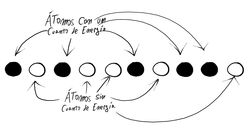
Suppose we have a system composed of 10 atoms. Each atom can only store 1 or 0 units of energy, referred to as energy quanta. How many distinct ways can these quanta be distributed if we have (a) 10 energy quanta and (b) 5 energy quanta?

Solution

We represent the atoms as spaces available for storing an energy quantum. If a space is filled, it means the corresponding atom already has its quantum of energy.

To count the ways in which k energy quanta can be distributed among n spaces, we use the combinatorial number:

\displaystyle \binom{n}{k}=\dfrac{n!}{k!(n-k)!}

This calculation gives us the number \Omega of possible states.

(a) If there are 10 quanta distributed among 10 spaces, there is only one way to do it. Thus, \Omega=1:

\displaystyle \Omega = \binom{10}{10}=\dfrac{10!}{10!(10-10)!} = \dfrac{10!}{10!0!} = 1

(b) For 5 quanta distributed among 10 spaces, we calculate:

\begin{array}{rl} \Omega &= \displaystyle\binom{10}{5} \\ \\ &=\dfrac{10!}{5!(10-5)!} = \dfrac{10!}{5!\cdot 5!} \\ \\ &= \dfrac{5! \cdot 6\cdot 7\cdot 8 \cdot 9\cdot 10}{5! \cdot 2\cdot 3\cdot 4\cdot 5} \\ \\ &= \dfrac{ 7\cdot 8 \cdot 9\cdot 10}{ 4\cdot 5} = 7\cdot 2 \cdot 9 \cdot 2 = 252 \end{array}

Therefore, there are 252 possible configurations.

Problems with Large Numbers

What we have analyzed so far is just the beginning. If we expand the system from case (b) to 100 atoms and 50 quanta, we obtain \Omega \approx 10^{28}. Now, imagine performing the same calculation with a mole of atoms; the result would be inconceivable.

Using Logarithms and Stirling’s Formula to Estimate Orders of Magnitude

When we want to estimate a magnitude of the form \Omega = \binom{n}{k} for large values of n, especially when k=n/2, which is the case where maximum values are reached, it is useful to employ Stirling’s logarithmic approximation.

To manage numbers of this magnitude, we can reformulate the calculations by taking logarithms, yielding:

\displaystyle \ln(\Omega)=\ln\left(\dfrac{n!}{k!(n-k)!}\right)= \ln(n!) - \ln((n-k)!) - \ln(k!)

This expression can be refined using Stirling’s approximation for the logarithm of factorials. There are two possible versions of the approximation:

• Ordinary approximation: \ln(n!) \approx \dfrac{1}{2}\ln(2n\pi) + n\ln(n) - n
• Simplified approximation: \ln(n!) \approx n\ln(n) - n

Development via Simplified Approximation

Using the simplified approximation, we obtain the following results:

\begin{array}{rl} \ln(\Omega) & \approx n\ln(n) - n - (n-k)\ln(n-k) + (n-k) - k\ln(k) + k \\ \\ &= n\ln(n) - (n-k)\ln(n-k) - k\ln(k) \\ \\ &= n\ln(n) - n\ln(n-k) + k\ln(n-k) - k\ln(k) \\ \\ &= \ln\left[ \left( \dfrac{n}{n-k} \right)^n \right] + k\ln\left( \dfrac{n-k}{k} \right) \\ \\ &= \ln\left[ \dfrac{1}{\left(1 - \dfrac{k}{n} \right)^n} \right] + k\ln\left( \dfrac{n}{k} - 1 \right) \end{array}

Since this approximation considers large values of n, we apply the relation:

\displaystyle \lim_{n\to\infty} \left(1-\dfrac{k}{n} \right)^n = e^{-k}

Thus:

\ln(\Omega) \approx \ln(e^k) + k\ln\left( \dfrac{n}{k} -1 \right) = k + k\ln\left( \dfrac{n}{k} -1 \right)

Finally, by applying a base change for logarithms, we obtain:

\log(\Omega) = \log(e)\ln(\Omega) \approx k\log(e)\left[1 + \ln\left( \dfrac{n}{k} - 1 \right) \right]

This leads to the result:

\boxed{\Omega \approx 10^{k\log(e)\left[1 + \ln\left( \dfrac{n}{k} - 1 \right) \right]}}

Although this result does not provide the exact value of \Omega, it allows us to estimate the number of digits required to represent it, improving as n grows larger. With this method, it is sufficient to compute the exponent, which most calculators can handle.

Additionally, this approach quickly estimates the maximum value of \Omega for a large n. Considering the case where k=n/2, we obtain:

\text{Max}\left(\Omega\right) \approx 10^{\dfrac{n}{2}\log(e)\left[1 + \ln\left( \dfrac{n}{n/2} - 1 \right) \right]} = 10^{ n\log(e)/2 }

Development via Ordinary Approximation

While development using the ordinary approximation will yield a more precise result, it will involve additional calculations, leading to approximately equivalent results for large values of n. The development of this approximation recycles several calculations already performed in the simplified approximation, as shown in the following reasoning:

\begin{array}{rcl} \ln(\Omega) & = & \ln\left(\dfrac{n!}{k!(n-k)!}\right)= \ln(n!) - \ln((n-k)!) - \ln(k!) \\ \\ & \approx & \color{red}\dfrac{1}{2}\ln(2n\pi)\color{black} + n\ln(n) - n \\ \\ & & \color{red}-\dfrac{1}{2}\ln(2(n-k)\pi)\color{black} - (n-k)\ln(n-k) + (n-k) \\ \\ & & \color{red}-\dfrac{1}{2}\ln(2k\pi)\color{black} - k\ln(k) + k \end{array}

The portion highlighted in red corresponds to the additional elements considered in the ordinary approximation, while everything else was already derived in the simplified approximation. Based on this, we have:

\begin{array}{rcl} \ln(\Omega) & \approx & \color{red}\dfrac{1}{2}\ln\left( \dfrac{2n\pi}{2(n-k)\pi \cdot 2k\pi} \right)\color{black} + k + k\ln\left(\dfrac{n}{k} - 1\right) \\ \\ & = & k + k\ln\left(\dfrac{n}{k} - 1\right) - \dfrac{1}{2}\ln\left(\dfrac{2k\pi(n-k)}{n}\right) \end{array}

Then, using a logarithmic base change, we have:

\log(\Omega) = \log(e)\ln(\Omega) \approx \log(e) \left[ k + k\ln\left(\dfrac{n}{k} - 1\right) - \dfrac{1}{2}\ln\left(\dfrac{2k\pi(n-k)}{n}\right) \right]

Finally, taking the exponential with base 10, we get:

\Omega \approx 10^{\log(e) \left[ k + k\ln\left(\dfrac{n}{k} - 1\right) - \dfrac{1}{2}\ln\left(\dfrac{2k\pi(n-k)}{n}\right) \right]}

Now, similarly to before, we can find the maximum value of this number by evaluating k=n/2, which in this case provides the following result:

\begin{array}{rcl} \text{Max}(\Omega) &\approx & 10^{\log(e) \left[ \dfrac{n}{2} + \dfrac{n}{2}\ln\left(\dfrac{n}{(n/2)} - 1\right) - \dfrac{1}{2}\ln\left(\dfrac{2(n/2)\pi(n-n/2)}{n}\right) \right]} \\ \\ & = & 10^{\log(e) \left[\dfrac{n}{2} - \dfrac{1}{2}\ln\left(\dfrac{n\pi}{2} \right) \right]} = 10^{\log(e)(n-\ln(n\pi/2))/2} \end{array}

Examples of Combinatorial and Order of Magnitude Calculations

Case 1: Large Factorials

Let us estimate the order of magnitude of \left(10^{50}\right)!, i.e., the number of digits required to write this number.

Solution

To perform this calculation, we use Stirling’s formula as follows:

\begin{array}{rl} \ln\left[ \left(10^{50}\right)! \right] &\approx 10^{50}\ln\left(10^{50}\right) - 10^{50}\\ \\ &= \left[\ln\left(10^{50}\right) -1\right]10^{50} \\ \\ &= \left[50\ln(10)-1 \right]10^{50} \\ \\ \end{array}

Next, we apply the base change for logarithms:

\ln\left[ \left(10^{50}\right)! \right] = \dfrac{\log\left[\left(10^{50}\right)!\right]}{\log{e}}

Thus:

\log\left[ \left(10^{50}\right)! \right] \approx \log(e)\left[50\ln(10)-1 \right]10^{50}

Finally, applying the base-10 exponential, we get:

\left(10^{50}\right)! \approx 10^{\log(e)\left[50\ln(10)-1 \right]10^{50}} = 10^{49,5657 \cdot 10^{50}}

The exponent on the 10 represents the order of magnitude, providing an estimate of the number of digits in the number \left(10^{50}\right)!.

Case 2: Large Combinations

An average house has approximately 12 light switches, which can be either on or off. On average, each house accommodates 4 people. If a city has 5 million inhabitants, how many possible ways are there for half of the city’s switches to be turned on?

Solution

The total number n of switches in the city is:

\begin{array}{rcl} n &=&\dfrac{\text{city inhabitants}}{\text{people per house}} \times \text{switches per house} \\ \\ &=& \dfrac{5\cdot 10^6}{4}\cdot 12 = 15\cdot 10^6 \end{array}

The macrostate formed by all microstates where half of the switches are on coincides with the macrostate that has the largest number of possible configurations. Denoting this maximum number as \Omega_{max}, we can estimate it using each method:

Ordinary Approximation: \Omega_{max} = 10^{\log(e)\left[15\cdot10^6 - \ln\left(15\pi\cdot10^6 / 2 \right) \right]/2} \approx 10^{6.514.413,542}
Simplified Approximation: \Omega_{max} = 10^{\log(e)\left[15\cdot10^6 \right]/2} \approx 10^{6.514.417,229}

Although there is a difference of nearly 4 orders of magnitude between the two approximations (which may seem significant), this is actually negligible compared to the over 6.5 million orders of magnitude involved.