Weierstrass Extreme Value Theorem
Why is it that in so many optimization problems it is almost taken for granted that “the maximum exists” or that “there is always a minimum” on a given interval, when in reality nothing forces that to be the case? The Weierstrass Theorem is the missing piece of that puzzle: it guarantees that a continuous function defined on a closed and bounded interval not only is bounded, but also actually attains its extreme values. In this entry we review its statement, build a detailed and rigorous proof based on pointwise continuity, compactness, and the supremum axiom, and comment on its modern interpretation in terms of continuous functions on compact sets. The aim is that, by the end, you do not merely recall the theorem as a sentence, but understand why it is true and why it appears repeatedly in analysis, optimization, and applied models.
Learning Objectives
- Understand the statement of the Weierstrass Theorem.
Identify precisely the hypotheses of the theorem (continuous function on a closed and bounded interval [a,b]) and its main conclusions: boundedness and the existence of maximum and minimum values. - Interpret the Weierstrass Theorem in terms of compactness.
Formulate the result in modern language: continuous functions map compact sets into sets where extreme values are attained, connecting the case of [a,b] with the broader framework of real analysis. - Relate the Weierstrass Theorem to optimization problems.
Recognize the role of the theorem as the theoretical foundation for the existence of maxima and minima in many single-variable optimization problems, in both theoretical and applied contexts.
TABLE OF CONTENTS:
Introduction
Statement of the Weierstrass Theorem
Proof
Step 1: Pointwise continuity on [a,b]
Step 2: Open cover associated with continuity
Step 3: Compactness of [a,b] and finite subcover
Step 4: Construction of a \delta independent of x_0 (uniform continuity)
Step 5: From uniform continuity to boundedness of f on [a,b]
Step 6: Existence of maximum and minimum values
Interpretation in terms of compactness and conclusion
Introduction
The Weierstrass Extreme Value Theorem is one of those results that, although it usually appears in the early units of Real Analysis, in fact silently supports a large portion of applied mathematics. Whenever in physics, economics, or statistics we speak of “maximizing” or “minimizing” a quantity subject to certain constraints, we are essentially relying on an idea very close to what this theorem guarantees: that a continuous function defined on a closed and bounded interval is not only bounded, but actually attains its extreme values.
Intuitively, it may seem “obvious” that if we draw a continuous curve over a segment [a,b], then there must exist a highest and a lowest point. However, it is enough to make small changes in the hypotheses for this intuition to fail dramatically: if we open the interval, if the function ceases to be continuous, or if the domain is not bounded, maxima and minima may simply disappear. The Weierstrass Theorem brings order to this intuition and tells us precisely when we can rely on it and why.
From a theoretical perspective, this theorem is the first serious encounter with the idea of compactness: in modern language, what it states is that a continuous function maps compact sets into compact sets. From a practical perspective, this translates into the existence of solutions for many one-dimensional optimization problems, and it will be a key component for later results such as the Mean Value Theorem and, ultimately, for calmly understanding the Fundamental Theorem of Calculus.
In this section we will state the Weierstrass Theorem and develop its proof in detail, relying on the notion of continuity on [a,b] and on the supremum axiom. The idea is that this text serves as a solid reference: both for studying the result itself and for returning to it whenever you need to use it in proving other theorems or in rigorously justifying the existence of maxima and minima in concrete problems.
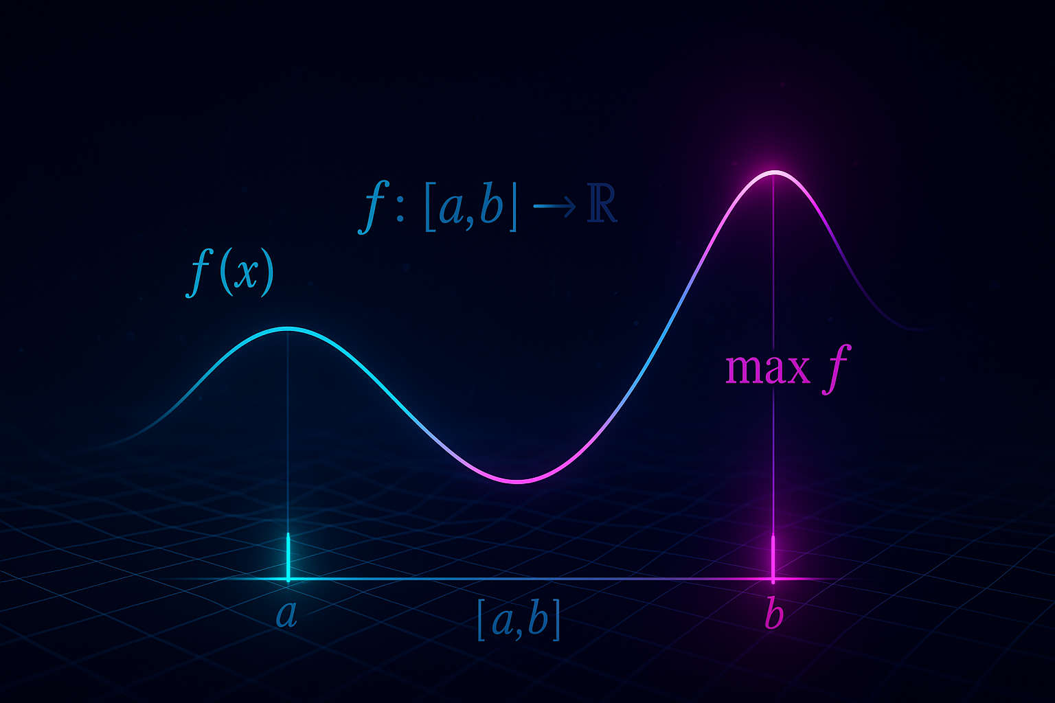
Statement of the Weierstrass Theorem
Every function f defined and continuous on [a,b], is bounded and has minimum and maximum values, m and M, such that if x\in[a,b], then f(x)\in[m,M]. |
Proof
Let us prove that if f:[a,b]\to\mathbb{R} is continuous on the closed and bounded interval [a,b], then f is bounded and attains a maximum and a minimum value on [a,b]. We will divide the proof into two major parts:
- First, we will show that the continuity of f on [a,b] implies that f is uniformly continuous, and from this we will deduce that it is bounded.
- Then, using the supremum axiom, we will prove that f attains its maximum and minimum values on the interval.
Step 1: Pointwise continuity on [a,b]
By hypothesis, f is continuous at every point x_0\in[a,b]. By the definition of continuity in terms of \epsilon and \delta, this means that:
\displaystyle (\forall x_0\in[a,b])(\forall \epsilon\gt 0)(\exists \delta(x_0)\gt 0) \big(|x-x_0|\lt\delta(x_0)\Rightarrow |f(x)-f(x_0)|\lt\epsilon\big).
At this point, the number \delta(x_0) may depend on the point x_0. Our immediate goal will be to construct, from these \delta(x_0), a single number \delta that does not depend on x_0 and that works simultaneously for all points in the interval.
Step 2: Open cover associated with continuity
Fix an arbitrary \epsilon\gt 0. For each x_0\in[a,b], the continuity of f allows us to choose a number \delta(x_0)\gt 0 such that
\displaystyle |x-x_0|\lt\delta(x_0)\Rightarrow |f(x)-f(x_0)|\lt\frac{\epsilon}{2}.
From these values we define, for each x_0\in[a,b], an open interval
\displaystyle I_{x_0}=\left(x_0-\frac{\delta(x_0)}{2},\,x_0+\frac{\delta(x_0)}{2}\right).
Each I_{x_0} is an open set in \mathbb{R} and, moreover, the family
\displaystyle \{I_{x_0}\}_{x_0\in[a,b]}
forms an open cover of [a,b]. Indeed, given any point y\in[a,b], it suffices to take x_0=y; by construction, y\in I_y. Thus, every point of the interval belongs to at least one of the open sets I_{x_0}.
This family of open sets is, in general, infinite (there is one for each x_0\in[a,b]). This is where the compactness of [a,b] comes into play.
Step 3: Compactness of [a,b] and finite subcover
We know from the Heine–Borel Theorem that a subset of \mathbb{R} is compact if and only if it is closed and bounded. The interval [a,b] is closed and bounded, therefore it is compact. By the definition of compactness, this means that:
From every open cover of [a,b] (even if it has infinitely many sets) one can extract a finite subcover.
Applying this property to the open cover \{I_{x_0}\}_{x_0\in[a,b]}, it follows that there exist points x_1,\dots,x_N\in[a,b] such that the corresponding intervals
\displaystyle I_{x_1},\, I_{x_2},\,\dots,\,I_{x_N}
they still cover the entire interval:
\displaystyle [a,b]\subset I_{x_1}\cup I_{x_2}\cup\cdots\cup I_{x_N}.
Thus, we have gone from an infinite family of open intervals to a subcover consisting of only a finite number of intervals, without losing the property of covering [a,b].
Step 4: Construction of a \delta that does not depend on x_0 (uniform continuity)
From the finite subcover we define the number
\displaystyle \delta=\min\left\{\frac{\delta(x_1)}{2},\frac{\delta(x_2)}{2},\dots,\frac{\delta(x_N)}{2}\right\}.
Since this is the minimum of a finite collection of positive numbers, we have \delta\gt 0. We will show that this \delta works for every point x_0\in[a,b], meaning it does not depend on the choice of x_0.
Now take:
- an arbitrary point x_0\in[a,b], and
- a point x\in[a,b] such that |x-x_0|\lt\delta.
Since the intervals I_{x_1},\dots,I_{x_N} cover [a,b], the point x_0 belongs to at least one of them, say to I_{x_j} for some j\in\{1,\dots,N\}. By the definition of I_{x_j}, this means that
\displaystyle |x_0-x_j|\lt\frac{\delta(x_j)}{2}.
Moreover, by the definition of \delta we have \delta\le\frac{\delta(x_j)}{2}, so from |x-x_0|\lt\delta it follows that
\displaystyle |x-x_0|\lt\frac{\delta(x_j)}{2}.
Applying the triangle inequality,
\displaystyle |x-x_j|\le |x-x_0|+|x_0-x_j| \lt \frac{\delta(x_j)}{2}+\frac{\delta(x_j)}{2} =\delta(x_j).
By the choice of \delta(x_j) (continuity of f at x_j for the value \epsilon/2), the inequalities |x_0-x_j|\lt\delta(x_j) and |x-x_j|\lt\delta(x_j) imply
\displaystyle |f(x_0)-f(x_j)|\lt\frac{\epsilon}{2} \quad\text{and}\quad |f(x)-f(x_j)|\lt\frac{\epsilon}{2}.
Using again the triangle inequality we obtain
\displaystyle |f(x)-f(x_0)| \le |f(x)-f(x_j)| + |f(x_j)-f(x_0)| \lt \frac{\epsilon}{2}+\frac{\epsilon}{2} =\epsilon.
Since x_0 and x were arbitrary, we have shown that for the \epsilon chosen at the beginning there exists a \delta\gt 0, independent of x_0, such that
\displaystyle (\forall x_0\in[a,b])(\forall x\in[a,b]) \big(|x-x_0|\lt\delta\Rightarrow |f(x)-f(x_0)|\lt\epsilon\big).
If we rename x_0 as y, this can be written as:
\displaystyle (\forall \epsilon\gt 0)(\exists \delta\gt 0)(\forall x,y\in[a,b]) \big(|x-y|\lt\delta\Rightarrow |f(x)-f(y)|\lt\epsilon\big),
which is precisely the definition of uniform continuity of f on [a,b]. In what follows, we will only need to apply this result to the case \epsilon=1.
Step 5: From uniform continuity to boundedness of f on [a,b]
Let us now apply uniform continuity with \epsilon=1. There exists a number \delta_1\gt 0 such that for all x,y\in[a,b] we have
\displaystyle |x-y|\lt\delta_1\Rightarrow |f(x)-f(y)|\lt 1.
We now divide the interval [a,b] into a finite number of subintervals whose length is smaller than \delta_1. That is, we choose an integer n and points
\displaystyle a = x_0 \lt x_1 \lt \cdots \lt x_n = b
such that for each k=0,1,\dots,n-1 we have
\displaystyle x_{k+1}-x_k\lt\delta_1.
We now consider the finite set of values
\displaystyle \{f(x_0),f(x_1),\dots,f(x_{n-1})\}.
Being a finite set of real numbers, we can define without issue
\displaystyle C = \max\{|f(x_k)| \;|\; k=0,1,\dots,n-1\}.
We will now show that C+1 is an upper bound in absolute value for f on the entire interval [a,b]. Let x\in[a,b] be an arbitrary point. Then there exists an index k such that x\in[x_k,x_{k+1}]. In particular,
\displaystyle |x-x_k|\le x_{k+1}-x_k\lt\delta_1.
By uniform continuity with \epsilon=1, from |x-x_k|\lt\delta_1 it follows that
\displaystyle |f(x)-f(x_k)|\lt 1.
Using the triangle inequality:
\displaystyle |f(x)|\le |f(x)-f(x_k)| + |f(x_k)| \lt 1 + |f(x_k)| \le 1 + C.
Since x\in[a,b] was arbitrary, we conclude that
\displaystyle |f(x)|\le C+1 \quad \text{for all } x\in[a,b],
that is, the function f is bounded on [a,b].
Step 6: Existence of maximum and minimum values
We define the set of values taken by the function on the interval:
\displaystyle H=\{f(x)\;|\;x\in[a,b]\}\subset\mathbb{R}.
We already know that H is nonempty (because [a,b] is nonempty) and bounded, so by the supremum axiom there exist real numbers
\displaystyle M=\sup H,\qquad m=\inf H.
Let us prove that M is attained as a value of the function, that is, that there exists x_1\in[a,b] with f(x_1)=M. We proceed by contradiction.
Suppose that f(x) never attains the value M, that is:
\displaystyle (\forall x\in[a,b])\big(f(x)\lt M\big).
Under this assumption, the function
\displaystyle g(x)=\frac{1}{M-f(x)}
is well defined and positive for all x\in[a,b], since by hypothesis M-f(x)\gt 0. Moreover, since f is continuous and M is constant, g is also continuous. By the first part of the proof, every continuous function on [a,b] is bounded, so there exists a number N\gt 0 such that
\displaystyle (\forall x\in[a,b])\big(g(x)\le N\big).
In particular, for all x\in[a,b] we have
\displaystyle \frac{1}{M-f(x)} = g(x)\le N,
which is equivalent to
\displaystyle M-f(x)\ge \frac{1}{N} \quad\Rightarrow\quad f(x)\le M-\frac{1}{N}.
This means that all values of f(x) on [a,b] are less than or equal to M-\frac{1}{N}. In particular, the supremum of H satisfies
\displaystyle \sup H\le M-\frac{1}{N}\lt M,
which contradicts the definition of M as the supremum of H. Therefore, our initial assumption was false, and there must exist a point x_1\in[a,b] such that
\displaystyle f(x_1)=M.
A completely analogous argument, applied to the infimum m=\inf H (for example, by considering the function h(x)=-f(x)), shows that there exists a point x_2\in[a,b] such that
\displaystyle f(x_2)=m.
Interpretation in terms of compactness and conclusion
We have proved that every continuous function f:[a,b]\to\mathbb{R} is bounded and attains its maximum and minimum values on [a,b]. In the modern language of analysis, this is interpreted by saying that in \mathbb{R}, closed and bounded intervals such as [a,b] are compact sets, and continuous functions map compact sets into compact sets.
In particular, if I is compact and f is continuous on I, then the image f(I) is a compact subset of \mathbb{R}. This guarantees that f(I) is bounded and that it actually attains a maximum and a minimum value, which is precisely the content of the Weierstrass Theorem.