Monte Carlo Simulation: My Management Projection February 2024 – October 2025
Assess and be transparent
At the close of a turbulent October, I ran a Monte Carlo Simulation to evaluate—using data—the quality of my management since I started investing with real capital on February 1, 2024. The observation window for this run ends on October 30, 2025. This exercise gives me an objective benchmark, the bar I want to clear in each iteration, and adds transparency for those who copy my portfolio on eToro.
Why Monte Carlo
Because it doesn’t guess; it translates what already happened into probabilities. From the monthly returns I estimate mean and volatility and, with those parameters, simulate thousands of plausible paths. This lets me audit my process with a criterion that is consistent and comparable over time.
Assumptions and limits
Trajectories are generated at a monthly frequency using parameters estimated on n=21 (Feb 2024→Oct 2025). The results are conditional on these data and assumptions; they do not constitute a prediction. To reflect uncertainty and tails, empirical bootstrap is employed (quantiles/CVaR), and percentile stability is reviewed with expanding out-of-sample windows. Any reading of risk should be considered in light of potential regime changes.
Monte Carlo Simulation
Input data
| Window | Observations | Monthly mean (μ) | Monthly volatility (σ) |
|---|---|---|---|
| Feb 1, 2024 to Oct 30, 2025 | 21 | 1.69 % | 3.51 % |
If you want to see more specific details about my returns and portfolio, check my eToro profile.
Simulation parameters
| Horizon | Months | Iterations | Bands shown | Baseline | Frequency |
|---|---|---|---|---|---|
| 5 years | 60 | 1000 | 50% (P25–P75), 80% (P10–P90), 90% (P05–P95) | Initial factor = 1 | Monthly |
| 10 years | 120 | 5000 | 50% (P25–P75), 80% (P10–P90), 90% (P05–P95) | Initial factor = 1 | Monthly |
Simulation results
The simulation outlines a central growth path consistent with the improvement observed between 2024 and 2025. The projected median trends upward and the typical bands remain contained, suggesting that the current method is generating returns with good stability for the level of risk taken.
- Upward consistency: the central pattern of the paths matches the year-over-year improvement in the sample
(approximate monthly mean 1.20 % in 2024 versus 2.22 % in 2025 and a higher frequency of positive months). This supports that recent execution was stronger. - Bounded risk: negative tails remain moderate at the 5- and 10-year horizons. The conservative scenario keeps cumulative growth above zero, in line with a medium risk profile around 4 in 2025.
- Favorable skew: the fan shows right skew. There are high-outcome scenarios with low probability while the median holds, indicating that extraordinary months push upward without compromising the base.
- Relative performance validated: 2025 YTD outperforms major global indices, and the simulation suggests this performance does not depend on a single exceptional month, but on a distribution of results consistent with the sample.
- Operational implication: maintain the discipline of rebalancing and no leverage. For the next update, the goal is to lift the median and narrow the P25–P75 band, with specific attention to the 5th percentile as an indicator for controlling infrequent drawdowns.


Elements to consider going forward
The current constraint is sample size; as more months are observed, estimates stabilize (error falls ~1/√n) and the simulation becomes more reliable. This can be improved by re-estimating with a rolling window that incorporates each new month and by applying shrinkage toward a benchmark while n is small, so the anchor loses weight as evidence grows and the variability of the mean and volatility decreases without overfitting. The treatment of tails and quantiles can also be improved: with more observations, percentiles and CVaR become less unstable; this is achieved via empirical bootstrap to quantify quantile uncertainty and, when exceedances are sufficient, with extreme value theory (peaks over threshold) to better anchor rare events. Temporal dependence can be captured more accurately because a longer series allows lower-error estimates of autocorrelation and volatility dynamics; here it is useful to use block bootstrap (block size guided by the ACF) or a simple GARCH and simulate from residuals to reproduce runs and clustering. The mixing of dissimilar periods is reduced by detecting regime changes: with more history, detectors gain power, parameters are estimated by regime, and scenarios are combined according to their probability, avoiding mixing bias. Finally, continuous calibration is strengthened by checking P5–P95 coverage and the PIT in expanding out-of-sample windows; in the presence of persistent deviations, assumptions are adjusted. With more months, these practices yield more honest scenario bands and operational metrics that are more stable and useful for decision-making.
Important note
This is not a forecast. If the market regime changes, the probabilities change too. What it does provide is a probabilistic framework of possible outcomes, with probabilities estimated at the time of the simulation and valid under the market conditions in which the data were obtained. It is a reference to compare my management over time, not a guarantee.