Introduction

So far, we have examined in detail how Lorentz transformations are carried out, that is, how the coordinates in Minkowski spacetime of a specific event are altered when observed from different inertial reference frames. Next, we will review a different perspective for these developments, visualizing them as spacetime rotation transformations. We will soon discover that this approach provides algebraic advantages, generally simplifying calculations, especially when combining several consecutive Lorentz transformations.

Rotations in Minkowski Spacetime

Let’s start by analyzing how various spatial rotations are carried out in Minkowski spacetime. Since this is a four-dimensional space, the most practical way to establish a rotation is to do so with respect to a specific plane. Thus, we can define rotations on the xy planes, xz, and yz, as well as on the xt, yt, and zt planes. Rotations carried out in planes formed by spatial axes are purely spatial rotations, while those performed in planes composed of space and time axes are spacetime rotations. For now, we will focus on understanding purely spatial rotations in detail and then extend this knowledge to spacetime rotations.

Pure Spatial Rotations

Let’s begin our study of spatial rotations by reviewing how rotations are performed in the xy plane. To do this, let’s assume we have a point with coordinates (a,b) with respect to the system defined by the \hat{x} and \hat{y} axes. Next, we will analyze the relationship that connects these coordinates with those observed by a rotated reference system. This system is defined by the \hat{x}^\prime and \hat{y}^\prime axes, which are rotated by an angle \theta with respect to the original system, as shown in the following figure:

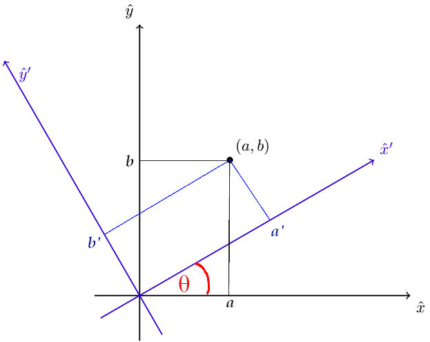
To obtain the relationships between the coordinates (a,b) and (a^\prime,b^\prime) measured from each system, we can use the following guide lines:

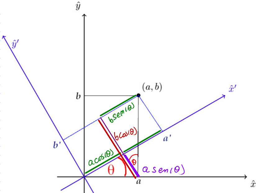
Thus, it is now easy to obtain the transformation equations

\begin{array}{rcl} a^\prime & = & \phantom{-}a\cos(\theta) + b\sin(\theta) \\ b^\prime & = & -a \sin(\theta) + b \cos(\theta) \end{array}

Matrix Generalization for Three-Dimensional Rotations

This system of equations can be more conveniently represented in its matrix form.

\left(\begin{array}{r} a^\prime \\ b^\prime \end{array}\right) = \left(\begin{array}{cc} \cos(\theta) & \sin(\theta) \\ -\sin(\theta) & \cos(\theta)\end{array}\right) \left(\begin{array}{r} a \\ b \end{array}\right)

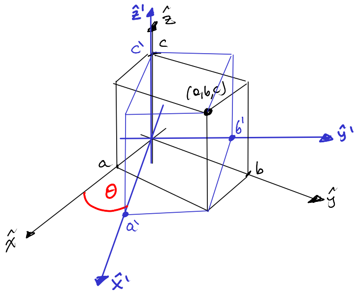
This is convenient because from here it is easy to generalize to larger dimensions. For example, a point with coordinates (a,b,c) in the system formed by the axes \hat{x}, \hat{y}, and \hat{z}, observed from another system formed by the axes \hat{x}^\prime, \hat{y}^\prime, and \hat{z}^\prime, which is distinguished from the original system by a rotation at an angle \theta with respect to the \hat{x}\hat{y} plane, would be:

\left(\begin{array}{r} a^\prime \\ b^\prime \\ c^\prime \end{array}\right) = \left(\begin{array}{ccc} \cos(\theta) & \sin(\theta) & 0 \\ -\sin(\theta) & \cos(\theta) & 0 \\ 0 & 0 & 1\end{array}\right) \left(\begin{array}{r} a \\ b \\ c\end{array}\right)

From this, we obtain the different rotation transformation matrices for each of the spatial planes.

\begin{array}{rll} R_{xy}(\theta)= & \left(\begin{array}{ccc} \cos(\theta) & \sin(\theta) & 0 \\ -\sin(\theta) & \cos(\theta) & 0 \\ 0 & 0 & 1\end{array}\right) & \begin{array}{l} \text{Rotation at an angle }\theta\\ \text{on the }xy \text{plane} \end{array} \\ \\ R_{yz}(\theta)= & \left(\begin{array}{ccc} 1 & 0 & 0 \\ 0 & \cos(\theta) & \sin(\theta) \\ 0 & -\sin(\theta) & \cos(\theta)\end{array}\right) & \begin{array}{l} \text{Rotation at an angle }\theta\\ \text{on the }yz \text{plane} \end{array} \\ \\ R_{xz}(\theta)= & \left(\begin{array}{ccc} \cos(\theta) & 0 & \sin(\theta) \\ 0 & 1 & 0 \\ -\sin(\theta) & 0 & \cos(\theta)\end{array}\right) & \begin{array}{l} \text{Rotation at an angle }\theta\\ \text{on the }xz \text{plane} \end{array} \end{array}

To calculate the inverse transformation of these rotation transformations, just substitute \theta with -\theta.

Spatial Rotations for Events with Spacetime Coordinates

Similarly to how we generalized from two to three dimensions, we can extend this to four dimensions. To remain consistent with the language of special relativity, it is important to understand the meaning of each coordinate. Generally, spacetime coordinates are expressed as follows:

x^\mu = (x^0, x^1, x^2, x^3) = (ct, x, y, z)

Here, the superscripts do not denote powers but indicate the characteristics of each coordinate. The coordinate with superscript 0 represents the temporal dimension, while the coordinates with superscripts 1, 2, and 3 correspond to the spatial dimensions. With this in mind, purely spatial rotations in Minkowski spacetime are described by the following relationships:

Rotation with respect to the xy plane: \underbrace{\left(\begin{array}{r} x^{\prime 0} \\ x^{\prime 1} \\ x^{\prime 2} \\ x^{\prime 3} \end{array}\right)}_{\large{x^{\prime \mu}}} = \underbrace{\left(\begin{array}{cccc} 1 & 0 & 0 & 0 \\ 0 & \cos(\theta) & \sin(\theta) & 0 \\ 0 & -\sin(\theta) & \cos(\theta) & 0 \\ 0 & 0 & 0 & 1 \end{array}\right)}_{\large{{R_{xy}(\theta)^\mu}_\nu}} \underbrace{\left(\begin{array}{c} x^0 \\ x^1 \\ x^2 \\ x^3 \end{array}\right)}_{\large{x^{\nu}}}

Rotation with respect to the yz plane: \underbrace{\left(\begin{array}{c} x^{\prime 0} \\ x^{\prime 1} \\ x^{\prime 2} \\ x^{\prime 3} \end{array}\right)}_{\large{x^{\prime \mu}}} = \underbrace{\left(\begin{array}{cccc} 1 & 0 & 0 & 0 \\ {} 0 & 1 & 0 & 0 \\ 0 & 0 & \cos(\theta) & \sin(\theta) \\ 0 & 0 & -\sin(\theta) & \cos(\theta) \end{array}\right)}_{\large{{R_{yz}(\theta)^\mu}_\nu}} \underbrace{\left(\begin{array}{r} x^0 \\ x^1 \\ x^2 \\ x^3 \end{array}\right)}_{\large{x^{\nu}}}

Rotation with respect to the xz plane: \underbrace{\left(\begin{array}{c} x^{\prime 0} \\ {}x^{\prime 1} \\ x^{\prime 2} \\ x^{\prime 3} \end{array}\right)}_{\large{x^{\prime \mu}}} = \underbrace{\left(\begin{array}{cccc} 1 & 0 & 0 & 0 \\ 0 & \cos(\theta) & 0 & \sin(\theta) \\ 0 & 0 & 1 & 0 \\ 0 & -\sin(\theta) & 0 & \cos(\theta) \end{array}\right)}_{\large{{R_{xz}(\theta)^\mu}_\nu}} \underbrace{\left(\begin{array}{r} x^0 \\ {} x^1 \\ x^2 \\ x^3 \end{array}\right)}_{\large{x^{\nu}}}

These transformations maintain exactly the same properties as their three-dimensional counterparts.

Hyperbolic Rotations of Spacetime

Introducing the Velocity Parameter

The similarity between Lorentz transformations and a spatial rotation can be obtained by introducing what we call the velocity parameter

\psi_{ss^\prime_x}= \text{argtanh}(\beta_{ss^\prime_x}).

Since \beta_{ss^\prime_x}\in]-1,1[, we have \psi_{ss^\prime_x}\in\mathbb{R}. Also note that, from this we will have that \gamma_{ss^\prime_x}=\cosh(\psi_{ss^\prime_x}) and \gamma_{ss^\prime_x} \beta_{ss^\prime_x} = \sinh(\psi_{ss^\prime_x}). This is obtained from the following calculations:

It is clear that \psi_{ss^\prime_x}= \text{argtanh}(\beta_{ss^\prime_x}) is equivalent to saying \beta_{ss^\prime_x} =\tanh(\psi_{ss^\prime_x}); and therefore:

\begin{array}{rl} \gamma^2_{ss^\prime_x} &= \dfrac{1}{1-\beta^2_{ss^\prime_x}} \\ \\ & = \dfrac{1}{1-\tanh^2(\psi_{ss^\prime_x})} \\ \\ {} & = \dfrac{\cosh^2(\psi_{ss^\prime_x})}{\cosh^2(\psi_{ss^\prime_x}) - \sinh^2(\psi_{ss^\prime_x})} \\ \\ & = \cosh^2(\psi_{ss^\prime_x}) \end{array}

Since both the gamma factor and the hyperbolic cosine are always greater than or equal to 1, it is finally demonstrated that \gamma_{ss^\prime_x} = \cosh(\psi_{ss^\prime_x}).

Similarly, continuing the calculations made previously, we have:

\gamma^2_{ss^\prime_x} \beta^2_{ss^\prime_x} = \cosh^2(\psi_{ss^\prime_x}) \tanh^2(\psi_{ss^\prime_x})= \sinh^2(\psi_{ss^\prime_x}).

Therefore, \gamma_{ss^\prime_x} \beta_{ss^\prime_x} = \sinh(\psi_{ss^\prime_x}).

Formulating Spacetime Rotations as Hyperbolic Rotations

Having reached this point, we can now rewrite the factor associated with the velocity boost and the gamma factor using the velocity parameter in Lorentz transformations. Considering two inertial systems S and S^\prime in standard configuration, where the second is applied a boost on the x axis, \beta_{ss^\prime_x}, we have:

\begin{array}{rl} ct^\prime &= \gamma_{ss^\prime_x}(ct - \beta_{ss^\prime_x} x) \\ &= \gamma_{ss^\prime_x} ct - \gamma_{ss^\prime_x}\beta_{ss^\prime_x} x \\ &= ct\cosh(\psi_{ss^\prime_x}) - x\sinh(\psi_{ss^\prime_x}), \\ \\ x^\prime &= \gamma_{ss^\prime_x}(x - \beta_{ss^\prime_x} ct) \\ &= -\gamma_{ss^\prime_x}\beta_{ss^\prime_x} ct + \gamma_{ss^\prime_x}x \\ &= -ct \sinh(\psi_{ss^\prime_x}) + x\cosh(\psi_{ss^\prime_x}), \\ \\ y^\prime &= y, \\ \\ z^\prime &= z. \end{array}

This system of equations allows the following matrix representation:

Hyperbolic Rotation of Spacetime on the tx Plane:

\begin{array}{rl} \underbrace{\left( \begin{array}{c} ct^\prime \\ x^\prime \\ y^\prime \\ z^\prime \end{array} \right)}_{\large{x^{\prime \mu}}} &= \underbrace{\left( \begin{array}{cccc} \cosh(\psi_{ss^\prime_x}) & -\sinh(\psi_{ss^\prime_x}) & 0 & 0 \\ - \sinh(\psi_{ss^\prime_x}) & \cosh(\psi_{ss^\prime_x}) & 0 & 0 \\ {} 0 & 0 & 1 & 0 \\ 0 & 0 & 0 & 1 \end{array}\right)}_{\large{{R_{tx}(\psi_{ss^\prime_x})^\mu}_\nu}} \underbrace{\left( \begin{array}{c} ct \\ x \\ y \\ z \end{array} \right)}_{\large{x^{\nu}}} \end{array}

Similarly, we have hyperbolic rotations on each of the spacetime planes:

Hyperbolic Rotation of Spacetime on the ty Plane:

\begin{array}{rl} \underbrace{\left( \begin{array}{c} ct^\prime \\ x^\prime \\ y^\prime \\ z^\prime \end{array} \right)}_{\large{x^{\prime \mu}}} &= \underbrace{\left(\begin{array}{cccc} \cosh(\psi_{ss^\prime_y}) & 0 & -\sinh(\psi_{ss^\prime_y}) & 0 \\ 0 & 1 & 0 & 0 \\ {} - \sinh(\psi_{ss^\prime_y}) & 0 & \cosh(\psi_{ss^\prime_y}) & 0 \\ 0 & 0 & 0 & 1 \end{array}\right)}_{\large{{R_{ty}(\psi_{ss^\prime_y})^\mu}_\nu}} \underbrace{\left( \begin{array}{c} ct \\ x \\ y \\ z \end{array} \right)}_{\large{x^{\nu}}} \end{array}

Hyperbolic Rotation of Spacetime on the tz Plane:

\begin{array}{rl} \underbrace{\left( \begin{array}{c} ct^\prime \\ x^\prime \\ y^\prime \\ z^\prime \end{array} \right)}_{\large{x^{\prime \mu}}} &= \underbrace{\left( \begin{array}{cccc} \cosh(\psi_{ss^\prime_x}) & -\sinh(\psi_{ss^\prime_x}) & 0 & 0 \\ - \sinh(\psi_{ss^\prime_x}) & \cosh(\psi_{ss^\prime_x}) & 0 & 0 \\ {} 0 & 0 & 1 & 0 \\ 0 & 0 & 0 & 1 \end{array}\right)}_{\large{{R_{tx}(\psi_{ss^\prime_x})^\mu}_\nu}} \underbrace{\left( \begin{array}{c} ct \\ x \\ y \\ z \end{array} \right)}_{\large{x^{\nu}}} \end{array}

Due to their form and algebraic properties, these transformations are very similar to a spatial rotation, except that instead of using trigonometric functions, they use hyperbolic functions. Although they are not rotations in the strict sense, they maintain some analogy with the rotations reviewed at the beginning. For example, similar to what happens with rotations, the inverse transformation is obtained by replacing the corresponding velocity parameter \psi with -\psi. These transformations are sometimes called hyperbolic rotations, and the velocity parameter is also known as the hyperbolic angle.