
Limit of Functions of a Real Variable
Summary:
This class thoroughly reviews the formal definition of limits of functions of a real variable, and from this, the main properties that lead to the algebra of limits are demonstrated.
Learning Objectives:
At the end of this class, the student will be able to:
- Recall the definition of limits of functions of a real variable.
- Demonstrate the properties that lead to the algebra of limits through \epsilon-\delta deductions.
- Calculate limits of functions of a real variable using the algebra of limits and its properties.
CONTENT INDEX
Introduction
The Intuitive Notion of Limit of a Function from a Graphical Approach
The Formal Definition of Limit
Properties of Limits
If the Limit Exists, Then It Is Unique
Algebra of Limits
Calculation of Simple Limits
Introduction
What is the difference between studying algebra and geometry compared to the study of calculus? The answer to this question is given by the concept of limit. Therefore, in this article, the limit and its definition are studied.
We usually associate the word “limit” with some kind of boundary, like the boundary of an interval with endpoints a, b (independent of its nature)
[a,b[\;\; ;\;\; ]a,b]\;\; ; \;\; ]a,b[\;\; ; [a,b] ,
or like the present, which we can say is the boundary between the past and the future. In a more or less similar way, the idea of limit introduces the mathematical understanding of this intuitive idea of approaching a certain point asymptotically.
The Intuitive Notion of Limit of a Function from a Graphical Approach
To start visualizing the idea of limit, it is helpful to begin with the graphical representation of a function and ask what will happen to f(x) as x approaches x_0 as closely as desired.
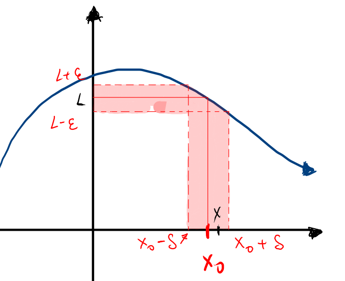
If x is close to x_0, then there will be an open interval of radius \delta and center x_0 such that x is contained within it. We can represent this in three different ways:
|x-x_0|\lt \delta,
|x\in]x_0 - \delta , x_0 + \delta[ ,
or x\in\mathcal{B}(x_0,\delta)
In our context, these are three ways of saying the same thing; although the last one, which reads as “the x contained in the open ball of center x_0 and radius \delta, would be more suitable for a topology course, where this “proximity topic” would be explored in more depth.
If this occurs, we will observe that there will be another open interval centered at l with radius \epsilon such that f(x) is contained within it, i.e., |f(x) - l|\lt \epsilon.
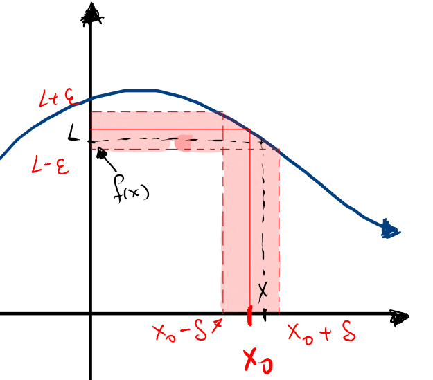
From here, the basic idea of the mathematical concept of limit emerges, from the fact that this will exist when: if 0 \lt|x-x_0|\lt \delta, then |f(x)-l|\lt \epsilon; and this value l will be the limit of the function as x approaches x_0 as closely as we want.
The Formal Definition of Limit
From the intuitive and graphical conception just presented, we can begin to uncover the formal definition of limit. We say that the limit exists when, no matter what this \epsilon is (i.e., the distance between f(x) and l), there will always exist a \delta such that, if 0 \lt|x-x_0|\lt \delta then |f(x) - l|\lt \epsilon. This idea, which is initially difficult to grasp and brings tears to most calculus students worldwide, can be summarized through the following expression:
\displaystyle \lim_{x\to x_0}f(x)=l := \left(\forall \epsilon \gt 0\right)\left(\exists \delta\gt 0\right) \left(0 \lt|x-x_0|\lt\delta \rightarrow |f(x) - l|\lt \epsilon\right),
Properties of Limits
The importance of having a formal definition of limits is that now, based on this, we can demonstrate its properties, both those that are intuitive and others that are not so much.
Before continuing, while it is not strictly necessary, it is highly recommended that you review some concepts of mathematical logic so that you can more easily understand the demonstrations that follow.
If the limit exists, then it is unique
To demonstrate this property, we will use the technique of proof by contradiction. We will start by defining the following set of premises:
\displaystyle\mathcal{H}= \{\lim_{x\to x_0}f(x) = L, \lim_{x\to x_0}f(x) = L^\prime, L\neq L^\prime\}.
From this, we can construct the following formal proof:
| (1) | \displaystyle \mathcal{H}\vdash \lim_{x\to x_0}f(x) = L ; Assumption |
| \displaystyle \mathcal{H}\vdash \left(\forall \epsilon \gt 0\right)\left(\exists \delta\gt 0\right) \left(0 \lt|x-x_0|\lt\delta \rightarrow |f(x) - L|\lt \epsilon\right) | |
| (2) | \displaystyle \mathcal{H}\vdash \lim_{x\to x_0}f(x) = L^\prime ; Assumption |
| \displaystyle \mathcal{H}\vdash \left(\forall \epsilon \gt 0\right)\left(\exists \delta\gt 0\right) \left(0 \lt|x-x_0|\lt\delta \rightarrow |f(x) - L^\prime |\lt \epsilon\right) | |
| (3) | \displaystyle \mathcal{H}\vdash L \neq L^\prime ; Assumption |
| (4) | \displaystyle \mathcal{H}\vdash \left(\forall \epsilon \gt 0\right)\left(\exists \delta\gt 0\right) \left(0 \lt|x-x_0|\lt\delta \rightarrow\right. \left. \left[ \left( |f(x) - L |\lt \epsilon \right) \wedge \left( |f(x) - L^\prime |\lt \epsilon\right) \right] \right. ); \wedge–Int(1,2) |
| (5) | \displaystyle \mathcal{H}\cup\{L\lt L^\prime\}\vdash \left(\forall \epsilon \gt 0\right)\left(\exists \delta\gt 0\right) \left(0 \lt|x-x_0|\lt\delta \rightarrow\right. \left. \left[ \left( |f(x) - L |\lt \epsilon \right) \wedge \left( |f(x) - L^\prime |\lt \epsilon\right) \right] \right. ); Monotonicity(4) |
| (6) | \displaystyle \mathcal{H}\cup\{L\lt L^\prime\}\vdash \epsilon = \frac{L - L^\prime}{2}\gt 0 ; Because L \lt L^\prime |
| (7) | \displaystyle \mathcal{H}\cup\{L\lt L^\prime\}\vdash \left(\exists \delta\gt 0\right) \left(0 \lt|x-x_0|\lt\delta \rightarrow\right. \left. \left[ \left( |f(x) - L |\lt \frac{L - L^\prime}{2} \right) \wedge \left( |f(x) - L^\prime |\lt \frac{L - L^\prime}{2}\right) \right] \right. ); Using(5,6) |
| \displaystyle \mathcal{H}\cup\{L\lt L^\prime\}\vdash (\exists \delta\gt 0) (0 \lt|x-x_0|\lt\delta \rightarrow [ ( 2 |f(x) - L |\lt L - L^\prime ) \wedge ( 2|f(x) - L^\prime |\lt L - L^\prime) ]) | |
| \displaystyle \mathcal{H}\cup\{L\lt L^\prime\}\vdash (\exists \delta\gt 0) (0 \lt|x-x_0|\lt\delta \rightarrow [ ( -L + L^\prime \lt 2 (f(x) - L )\lt L - L^\prime ) \wedge ( -L + L^\prime \lt 2(f(x) - L^\prime )\lt L - L^\prime) ]) | |
| \displaystyle \mathcal{H}\cup\{L\lt L^\prime\}\vdash (\exists \delta\gt 0) (0 \lt|x-x_0|\lt\delta \rightarrow [ ( -L + L^\prime \lt 2f(x) - 2L \lt L - L^\prime ) \wedge ( -L + L^\prime \lt 2f(x) - 2L^\prime \lt L - L^\prime) ]) | |
| \displaystyle \mathcal{H}\cup\{L\lt L^\prime\}\vdash (\exists \delta\gt 0) (0 \lt|x-x_0|\lt\delta \rightarrow [ ( L + L^\prime \lt 2f(x) \lt 3L - L^\prime ) \wedge ( -L + 3L^\prime \lt 2f(x) \lt L + L^\prime) ]) | |
| \displaystyle \mathcal{H}\cup\{L\lt L^\prime\}\vdash (\exists \delta\gt 0) (0 \lt|x-x_0|\lt\delta \rightarrow [ ( -L + 3L^\prime \lt 2f(x) \lt L + L^\prime) \wedge ( L + L^\prime \lt 2f(x) \lt 3L - L^\prime ) ]) | |
| (8) | \displaystyle \mathcal{H}\cup\{L\lt L^\prime\}\vdash \bot ; From(1,2,6,7) |
| (9) | \displaystyle \mathcal{H}\cup\{L\gt L^\prime\}\vdash \bot ; Same procedure as (8) |
| (10) | \displaystyle \mathcal{H}\vdash [(L\lt L^\prime) \vee (L\gt L^\prime)] \rightarrow \bot ; \vee-int(8,9) |
| (11) | \displaystyle \mathcal{H}\vdash [L\ \neq L^\prime] \rightarrow \bot ; Def(10) |
| (12) | \displaystyle \mathcal{H}\vdash \bot ; MP(3,11) |
| \displaystyle \left\{\lim_{x\to x_0}f(x) = L, \lim_{x\to x_0}f(x) = L^\prime, L\neq L^\prime\right\} \vdash \bot | |
| (13) | \displaystyle \left\{\lim_{x\to x_0}f(x) = L, \lim_{x\to x_0}f(x) = L^\prime \right\} \vdash \neg(L\neq L^\prime) ; Contradiction(12) |
| \displaystyle \left\{\lim_{x\to x_0}f(x) = L, \lim_{x\to x_0}f(x) = L^\prime \right\} \vdash L = L^\prime. |
From this proof, we see that if two limits exist, they must be equal, and therefore the limit is unique.
Algebra of Limits
With what we’ve seen so far, we have reviewed the essentials of the mathematical idea of a limit. But this alone is not nearly enough to perform calculations with it; only someone mad and craving suffering would use the definition of a limit for this purpose. To solve this problem, we will now work on techniques that will help us start calculating some limits.
Let x_0, \alpha, \beta, L, M \in \mathbb{R}, and let f and g be real functions such that:
\displaystyle \lim_{x\to x_0} f(x) = L
\displaystyle \lim_{x\to x_0} g(x) = M
Then the following properties hold:
Limit of the Sum and Difference of Functions
\displaystyle \lim_{x\to x_0} \left(\alpha f(x) \pm \beta g(x) \right) = \alpha L \pm \beta M
Proof:
Consider the set of premises \displaystyle\mathcal{H}=\left\{\lim_{x\to x_0} f(x) = L, \lim_{x\to x_0} g(x) = M \right\}, and from this, we can reason as follows:
| (1) | \displaystyle \mathcal{H}\vdash \lim_{x\to x_0}f(x) = L ; Assumption |
| \displaystyle \mathcal{H}\vdash \left(\forall \epsilon \gt 0 \right)\left(\exists \delta \gt 0 \right) \left(0 \lt |x-x_0|\lt \delta \rightarrow |f(x) - L|\lt \epsilon \right) | |
| \displaystyle \mathcal{H}\vdash \left(\forall \epsilon \gt 0 \right)\left(\exists \delta \gt 0 \right) \left(0 \lt |x-x_0|\lt \delta \rightarrow |\alpha||f(x) - L|\lt |\alpha|\epsilon \right) | |
| \displaystyle \mathcal{H}\vdash \left(\forall \epsilon \gt 0 \right)\left(\exists \delta \gt 0 \right) \left( 0 \lt|x-x_0|\lt \delta \rightarrow |\alpha f(x) - \alpha L|\lt |\alpha|\epsilon \right) | |
| (2) | \displaystyle \mathcal{H}\vdash \overline{\epsilon}:= |\alpha|\epsilon ; Def. |
| (3) | \displaystyle \mathcal{H}\vdash \left(\forall \overline{\epsilon} \gt 0 \right)\left(\exists \delta \gt 0 \right) \left(0 \lt |x-x_0|\lt \delta \rightarrow |\alpha f(x) - \alpha L|\lt \overline{\epsilon} \right) ; From(1,2) |
| \displaystyle \mathcal{H}\vdash \lim_{x\to x_0}\alpha f(x) = \alpha L | |
| (4) | \displaystyle \mathcal{H}\vdash \lim_{x\to x_0}g(x) = M ; Assumption |
| (5) | \displaystyle \mathcal{H}\vdash \lim_{x\to x_0}\beta g(x) = \beta M ; Similar to (3) |
| \displaystyle \mathcal{H}\vdash \left(\forall \overline{\overline{\epsilon}} \gt 0 \right)\left(\exists \delta \gt 0 \right) \left( 0 \lt |x-x_0|\lt \delta \rightarrow |\beta g(x) - \beta M|\lt \overline{\overline{\epsilon}} \right) | |
| (6) | \displaystyle \mathcal{H}\vdash \left(\forall \overline{\epsilon},\overline{\overline{\epsilon}} \gt 0 \right)\left(\exists \delta \gt 0 \right) \left(0 \lt |x-x_0|\lt \delta \rightarrow \left[|\alpha f(x) - \alpha L|+ |\beta g(x) - \beta M|\lt \overline{\epsilon}+ \overline{\overline{\epsilon}} \right] \right) ; from(3,5) |
| (7) | \displaystyle \mathcal{H}\vdash |\alpha f(x) - \alpha L + \beta g(x) - \beta M| \leq |\alpha f(x) - \alpha L|+ |\beta g(x) - \beta M| ; Triangle Inequality: (\forall x,y\in\mathbb{R})(|x+y|\leq |x|+|y|) |
| (8) | \displaystyle \mathcal{H}\vdash \left(\forall \overline{\epsilon},\overline{\overline{\epsilon}} \gt 0 \right)\left(\exists \delta \gt 0 \right) \left(0 \lt |x-x_0|\lt \delta \rightarrow |\alpha f(x) - \alpha L + \beta g(x) - \beta M| \lt \overline{\epsilon}+ \overline{\overline{\epsilon}} \right) ; from(6,7) |
| (9) | \epsilon^* := \overline{\epsilon} + \overline{\overline{\epsilon}}; Definition |
| (10) | \displaystyle \mathcal{H}\vdash \left(\forall \epsilon^* \gt 0 \right)\left(\exists \delta \gt 0 \right) \left(0 \lt |x-x_0|\lt \delta \rightarrow |\alpha f(x) + \beta g(x) - \alpha L - \beta M| \lt \epsilon^* \right) ; from(8,9) |
| \displaystyle \mathcal{H}\vdash \lim_{x\to x_0} (\alpha f(x) + \beta g(x)) = \alpha L + \beta M | |
| (11) | \gamma:= - \beta; Definition |
| (12) | \displaystyle \mathcal{H}\vdash \lim_{x\to x_0} (\alpha f(x) + \gamma g(x)) = \alpha L + \gamma M ; Analogy(10) |
| (13) | \displaystyle \mathcal{H}\vdash \lim_{x\to x_0} (\alpha f(x) - \beta g(x)) = \alpha L - \beta M ; from(11,12) |
| (14) | \displaystyle \mathcal{H}\vdash \lim_{x\to x_0} (\alpha f(x) \pm \beta g(x)) = \alpha L \pm \beta M ; from(10,13) |
Limit of the Product of Functions
\displaystyle \lim_{x\to x_0} \left( f(x) g(x) \right) = L M
This proof is a bit more difficult than the previous one, but nothing that we can’t solve with a few draconian tricks. Using the same set of premises \mathcal{H} from the previous proof, we can build the following reasoning:
| (1) | \displaystyle \mathcal{H}\vdash \overline{\epsilon} := \frac{|\epsilon|}{2(|M|+1)} \leq \frac{|\epsilon|}{2} ; Definition |
| (2) | \displaystyle \mathcal{H}\vdash \lim_{x\to x_0} f(x) = L ; Assumption |
| \displaystyle \mathcal{H}\vdash \left(\forall \overline{\epsilon} \gt 0 \right)\left(\exists \delta \gt 0 \right)\left(0 \lt |x-x_0|\lt \delta \rightarrow |f(x) - L| \lt \overline{\epsilon} = \frac{|\epsilon|}{2(|M|+1)}\right) ; Using (1) | |
| (3) | \displaystyle \mathcal{H}\vdash \overline{\overline{\epsilon}} := \frac{|\epsilon|}{2(|L|+1)} \leq \frac{|\epsilon|}{2}; Definition |
| (4) | \displaystyle \mathcal{H}\vdash \lim_{x\to x_0} g(x) = M ; Assumption |
| \displaystyle \mathcal{H}\vdash \left(\forall \overline{\overline{\epsilon}} \gt 0 \right)\left(\exists \delta \gt 0 \right)\left(0 \lt |x-x_0|\lt \delta \rightarrow |g(x) - M| \lt \overline{\overline{\epsilon}} = \frac{|\epsilon|}{2(|L|+1)}\right) ; Using (3) | |
| (5) | \displaystyle \mathcal{H}\vdash |f(x)| - |L| \lt |f(x) - L| \lt \overline{\epsilon} \lt 1 ; Triangle Inequality + Special case of \overline{\epsilon} |
| (6) | \displaystyle \mathcal{H}\vdash |f(x)|\lt 1 + |L| ; From (5) |
| (7) | \displaystyle \mathcal{H}\vdash |g(x)| - |M| \lt |g(x) - M| \lt \overline{\overline{\epsilon}} \lt 1 ; Triangle Inequality + Special case of \overline{\overline{\epsilon}} |
| (8) | \displaystyle \mathcal{H}\vdash |g(x)| \lt 1 + |M| ; From (7) |
| (9) | \displaystyle \mathcal{H}\vdash |f(x)g(x) - LM|=| f(x)g(x) - Mf(x) + Mf(x) - LM |; Add zero |
| \displaystyle \mathcal{H}\vdash |f(x)g(x) - LM|=| f(x)(g(x) - M) + M (f(x) - L) |; Factor | |
| (10) | \displaystyle \mathcal{H}\vdash |f(x)g(x) - LM|\leq | f(x)(g(x) - M)| + | M (f(x) - L) |; Triangle Inequality(9) |
| \displaystyle \mathcal{H}\vdash |f(x)g(x) - LM|\leq |f(x)||g(x) - M| + |M| |f(x) - L| | |
| (11) | \displaystyle \mathcal{H}\vdash |f(x)g(x) - LM|\lt (1 + |L|)|g(x) - M|+ |M|\overline{\epsilon}; From (5,6,10) |
| (12) | \displaystyle \mathcal{H}\vdash \left[ |g(x) - M|\lt \overline{\overline{\epsilon}} \right] \rightarrow \left[ (1+|L|)|g(x) - M| + |M|\overline{\epsilon} \lt (1+|L|)\overline{\overline{\epsilon}} + |M|\overline{\epsilon}\right]; From (11) |
| (13) | \displaystyle \mathcal{H}\vdash \left[ |g(x) - M|\lt \overline{\overline{\epsilon}} \right] \rightarrow \left[ (1+|L|)|g(x) - M| + |M|\overline{\epsilon} \lt (1+|L|)\frac{|\epsilon|}{2(|L|+1)} + |M|\frac{|\epsilon|}{2(|M|+1)}\right]; From (1,3,12) |
| \displaystyle \mathcal{H}\vdash \left[ |g(x) - M|\lt \overline{\overline{\epsilon}} \right] \rightarrow \left[ (1+|L|)|g(x) - M| + |M|\overline{\epsilon} \lt \frac{|\epsilon|}{2} + \frac{|\epsilon||M|}{2(|M|+1)} \lt \frac{|\epsilon|}{2}+ \frac{|\epsilon|}{2} = |\epsilon| \right] | |
| (14) | \displaystyle \mathcal{H}\vdash \left[ |g(x) - M|\lt \overline{\overline{\epsilon}} \right] \rightarrow \left[ |f(x)g(x) - LM|\lt |\epsilon| \right]; From (11,13) |
| (15) | \displaystyle \mathcal{H}\vdash (\forall \epsilon \gt 0 ) (\exists \delta \gt 0 ) \left(0 \lt |x-x_0|\lt \delta \rightarrow |f(x)g(x) - LM|\lt |\epsilon| \leq \epsilon \right) ; From (1,2,4,14) |
| \displaystyle \mathcal{H}\vdash \lim_{x\to x_0}f(x)g(x) = LM. |
Limit of the Constant Function
The limit of the constant function f(x)=c, is the constant c. That is:
\displaystyle \lim_{x\to x_0}c = c
Proof
The proof of this is actually simple, because it is essentially a tautology. It is already known that:
\displaystyle \lim_{x\to x_0}c = c := (\forall\epsilon\gt 0) (\exists \delta \gt 0)(0\lt|x-x_0|\lt \delta \rightarrow |c-c|\lt \epsilon)
But it happens that 0=|c-c|\lt \epsilon is a tautology for every positive epsilon, so the implication is also a tautology, and consequently, the expression \displaystyle \lim_{x\to x_0}c = c is also a tautology.
Limit of the Quotient of Functions
We are now ready to prove the rule for the limit of the quotient between two functions. It is:
\displaystyle \lim_{x\to x_0}\frac{f(x)}{g(x)}= \frac{L}{M}
Where, just like in the previous properties, we assume that the set of premises holds:
\displaystyle \mathcal{H}=\{\lim_{x\to x_0}f(x) = L, \lim_{x\to x_0}g(x) = M\}
Proof
Fortunately, we won’t need to perform more demonstrations like the ones we’ve done before, because now we can directly use those results to achieve our goals. But before that, let’s first prove that
\displaystyle \lim_{x\to x_0}\frac{1}{g(x)} = \frac{1}{M}
To prove this, it is enough to use the rule of the product limit and the limit of a constant function in combination, we just need to be careful that g(x) is not zero:
\displaystyle 1 = \lim_{x\to x_0}\left( 1 \right) \lim_{x\to x_0}\left( g(x) \cdot \frac{1}{g(x)} \right) = \lim_{x\to x_0}g(x) \cdot \lim_{x\to x_0} \frac{1}{g(x)} = M \cdot \lim_{x\to x_0} \frac{1}{g(x)}
Therefore: \displaystyle \lim_{x\to x_0} \frac{1}{g(x)} = \frac{1}{M}
Finally, by the rule of the product limit, we have:
\displaystyle \lim_{x\to x_0} \frac{f(x)}{g(x)} = \lim_{x\to x_0} f(x) \frac{1}{g(x)}= L \cdot\frac{1}{M} = \frac{L}{M}
This will hold as long as M is not zero.
Limit of a Natural Power
This property tells us that, if \displaystyle \lim_{x_0 \to x_0}f(x) = L, then it will hold that \displaystyle \left(\forall n \in \mathbb{N}\right) \left( \lim_{x\to x_0} \left( [f(x)]^n \right) = L^n \right). This can be proven by mathematical induction.
Proof:
- Case n=1: (initial step)
\displaystyle \lim_{x\to x_0} [f(x)]^1 = \lim_{x\to x_0} f(x) = L. This concludes the initial step ✅
- Case n=k: (inductive step)
Assuming that \displaystyle \lim_{x\to x_0} [f(x)]^k = L^k (Induction Hypothesis) holds, we will now check that \displaystyle \lim_{x\to x_0} [f(x)]^{k+1} = L^{k+1} holds as well.
We have: \displaystyle \lim_{x\to x_0} [f(x)]^{k+1} = \lim_{x\to x_0} \{f(x) [f(x)]^k\} = \lim_{x\to x_0}f(x) \lim_{x\to x_0} [f(x)]^{k} =L \lim_{x\to x_0} [f(x)]^{k}. The latter follows from the product limit rule proved earlier.
Then, by the induction hypothesis, we have \displaystyle \lim_{x\to x_0} [f(x)]^{k+1} = L \lim_{x\to x_0} [f(x)]^{k} =L\cdot L^k = L^{k+1}. This concludes the inductive step ✅
- Therefore: \displaystyle \left(\forall n \in \mathbb{N}\right) \left( \lim_{x\to x_0} \left( [f(x)]^n \right) = L^n \right).
Limit of an nth Root
Similarly to powers, it will hold that \displaystyle \left(\forall n \in \mathbb{N}\right) \left( \lim_{x\to x_0} \sqrt[n]{f(x)} = \sqrt[n]{L} \right)
Proof:
Using the power rule we just proved, we have that:
\displaystyle L= \lim_{x\to x_0} f(x)=\lim_{x\to x_0} \left[\sqrt[n]{f(x)}\right]^n = \left[ \lim_{x\to x_0} \sqrt[n]{f(x)}\right]^n
Therefore: \displaystyle \lim_{x\to x_0} \sqrt[n]{f(x)} =\sqrt[n]{L}.
Limit of Fractional Powers
With the combined powers of the last two proofs, we can conclude our final proof, which is: \displaystyle \left(\forall p,q\neq 0 \in \mathbb{Z}\right) \left( \lim_{x\to x_0} \left[f(x)\right]^{\frac{p}{q}} = L^{\frac{p}{q}} \right). , which is obtained thanks to the product rule, because \displaystyle [f(x)]^{\frac{p}{q}} =[\sqrt[q]{f(x)}]^p and \displaystyle L^{\frac{p}{q}} =[\sqrt[q]{L}]^p.
Limit \displaystyle \lim_{x\to x_0}x = x_0
With this demonstration, we conclude this series of proofs, and with this one and the previous ones, we will be able to calculate a large number of limits in an almost intuitive way.
It is easy to prove that \displaystyle \lim_{x\to x_0}x = x_0, because for this to hold, it is necessary that:
(\forall \epsilon \gt 0) (\exists \delta \gt 0)(0\lt |x-x_0|\lt \delta\rightarrow |x-x_0|\lt \epsilon)
According to the definition of Limit, for all epsilon there must exist at least one delta for which everything else holds; so it is enough to find one to verify that, indeed, the limit is as claimed. But this is actually obvious because any \delta\leq\epsilon satisfies such a condition. Therefore: \displaystyle \lim_{x\to x_0}x = x_0.
Simple Limit Calculations
Thanks to all these theorems that we have just reviewed, a wide variety of limits can now be calculated in a rather intuitive way, as if we simply evaluated the function. Here you can see some examples:
- {}\\ \begin{array}{rl} \displaystyle \lim_{x\to 2}(x^2 + 4x) & = \displaystyle \lim_{x\to 2}(x^2) + \lim_{x\to 2}(4x) \\ \\ & = \displaystyle \left(\lim_{x\to 2} x \right)^2 + 4\lim_{x\to 2} x \\ \\ & = (2)^2 + 8 = 12 \end{array}
- {} \\ \begin{array}{rl} \displaystyle \lim_{x\to 1}\left.\frac{(3x-1)^2}{(x+1)^3} \right. & = \displaystyle \frac{(3(1)-1)^2}{((1)+1)^3} \\ \\ & = \displaystyle \frac{4}{8} = \frac{1}{2} \end{array}
- {} \\ \begin{array}{rl} \displaystyle \lim_{x\to 2} \frac{x-2}{x^2 - 4} &= \displaystyle \lim_{x\to 2} \frac{x-2}{(x-2)(x+2)} \\ \\ & = \displaystyle \lim_{x\to 2} \frac{1}{x+2} = \dfrac{1}{4} \end{array}
- {} \\ \begin{array}{rl} \displaystyle \lim_{h\to 0} \frac{(x+h)^3-x^3}{h} &= \displaystyle \lim_{h\to 0} \frac{x^3 + 3x^2 h + 3xh^2 -x^3}{h} \\ \\ & = \displaystyle\lim_{h\to 0} \frac{3x^3 h + 3xh^2}{h} \\ \\ & = \displaystyle \lim_{h\to 0} 3x^2 + 3xh = 3x^2 \end{array}
- {} \\ \begin{array}{rl} \displaystyle \lim_{x\to 1} \frac{x-1}{\sqrt{x^2 + 3} - 2 } &=\displaystyle \lim_{x\to 1} \frac{x-1}{\sqrt{x^2 + 3} - 2 } \frac{\sqrt{x^2 + 3} + 2}{\sqrt{x^2 + 3} + 2} \\ \\ & =\displaystyle \lim_{x\to 1} \frac{(x-1)(\sqrt{x^2 + 3} + 2)}{(x^2 + 3) - 4 } \\ \\ & =\displaystyle \lim_{x\to 1} \frac{(x-1)(\sqrt{x^2 + 3} + 2)}{x^2 -1 } \\ \\ & =\displaystyle \lim_{x\to 1} \frac{(x-1)(\sqrt{x^2 + 3} + 2)}{(x-1)(x+1) } \\ \\ & =\displaystyle \lim_{x\to 1} \frac{\sqrt{x^2 + 3} + 2}{ x+1 } \\ \\ & =\displaystyle \frac{2+2}{2} =2 \end{array}