
実数変数関数の極限
要約:
この講義では、実数変数関数の極限の正式な定義を深く検討し、それに基づいて極限の代数につながる主要な性質を証明します。
学習目標:
この講義の終了時に学生は以下のことができるようになります:
- 実数変数関数の極限の定義を想起する。
- \epsilon-\deltaによる演繹を通じて、極限の代数につながる性質を証明する。
- 極限の代数とその性質を用いて、実数変数関数の極限を計算する。
内容目次
はじめに
関数の極限の直感的概念(グラフによるアプローチ)
極限の正式な定義
極限の性質
極限が存在するなら、それは一意である
極限の代数
単純な極限の計算
はじめに
代数学や幾何学を学ぶことと、微積分を学ぶこととの違いは何か? この問いに対する答えは、極限という概念によって明らかになります。本稿では極限とその定義について学びます。
「極限」という語は通常、境界のようなものを連想させます。たとえば、端点が a, b である区間の境界(その性質に関わらず)などです。
[a,b[\;\; ;\;\; ]a,b]\;\; ; \;\; ]a,b[\;\; ; [a,b] ,
あるいは現在という時間も、過去と未来の境界とみなすことができます。これとある程度似た形で、極限という概念は、ある点に漸近的に近づいていくという直感的なアイデアを数学的に理解するための枠組みを提供します。
グラフ的アプローチによる関数の極限の直感的概念
極限の概念を視覚的に理解し始めるためには、関数のグラフを描くことから始めるのが適切です。そして f(x) が、x が x_0 に限りなく近づくときにどのような挙動を示すかを考察します。
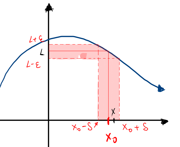
x が x_0 の近くにあるならば、中心 x_0、半径 \delta の開区間が存在して、x はその中に含まれます。このことは次の3通りの方法で表現できます:
|x-x_0|\lt \delta,
x\in]x_0 - \delta , x_0 + \delta[ ,
または x\in\mathcal{B}(x_0,\delta)
この文脈においては、これら3つは同じ内容を別の言い方で表しているに過ぎません。ただし最後の表現(中心 x_0、半径 \delta の開球に属する)は、位相空間論の講義などで「近接性」という概念をより深く扱う際に適しています。
このような状況下では、中心 l、半径 \epsilon の開区間が存在し、f(x) がその中に含まれる、すなわち:|f(x) - l|\lt \epsilon が成り立ちます。
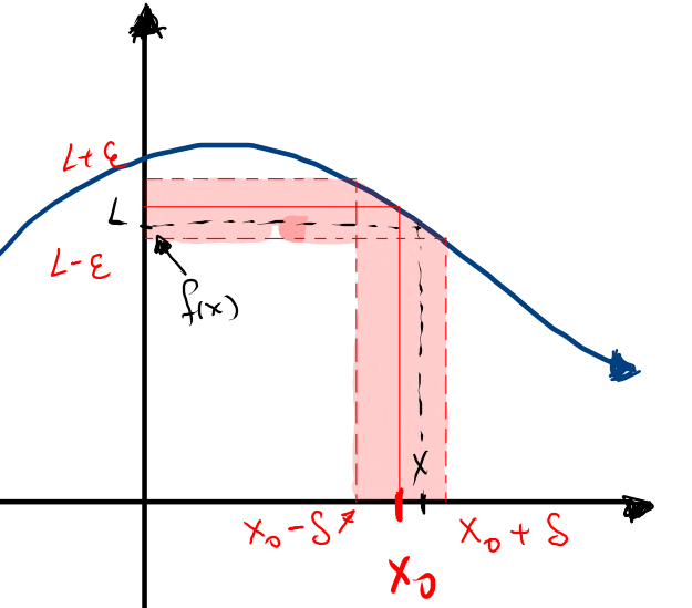
ここに、極限の数学的概念の根幹が現れます。それは以下の条件が成り立つときに極限が存在するということです:0 \lt|x-x_0|\lt \delta ならば |f(x)-l|\lt \epsilon。このとき、l は x が x_0 に限りなく近づくときの関数の極限値になります。
極限の正式な定義
上で提示された直感的かつ図的な理解から、極限の正式な定義を明確にすることができます。 極限が存在するとは、任意の \epsilon(すなわち、f(x) と l との距離)に対して、ある \delta が存在して、0 \lt|x-x_0|\lt \delta ならば |f(x) - l|\lt \epsilon が成り立つということです。この概念は最初は捉えにくく、世界中の多くの微積分の学生にとって涙の種となるものですが、次の表現で要約することができます:
\displaystyle \lim_{x\to x_0}f(x)=l := \left(\forall \epsilon \gt 0\right)\left(\exists \delta\gt 0\right) \left(0 \lt|x-x_0|\lt\delta \rightarrow |f(x) - l|\lt \epsilon\right),
極限の性質
極限の正式な定義を持つことの重要性は、そこから直感的なものもそうでないものも含めて、極限に関する性質を証明できるという点にあります。
ここから先へ進む前に、必須ではありませんが、以下のリンク先にある 数学論理 のいくつかの基本概念を復習しておくことを強く推奨します。そうすることで、これから出てくる証明をより容易に理解できるでしょう。
極限が存在するならば、それは一意である
この性質を証明するために、背理法(帰謬法)を用います。 まず、次の前提集合を定義するところから始めます:
\displaystyle\mathcal{H}= \{\lim_{x\to x_0}f(x) = L, \lim_{x\to x_0}f(x) = L^\prime, L\neq L^\prime\}.
これらの前提に基づいて、次の形式的な証明を構築できます:
| (1) | \displaystyle \mathcal{H}\vdash \lim_{x\to x_0}f(x) = L ; 仮定 |
| \displaystyle \mathcal{H}\vdash \left(\forall \epsilon \gt 0\right)\left(\exists \delta\gt 0\right) \left(0 \lt|x-x_0|\lt\delta \rightarrow |f(x) - L|\lt \epsilon\right) | |
| (2) | \displaystyle \mathcal{H}\vdash \lim_{x\to x_0}f(x) = L^\prime ; 仮定 |
| \displaystyle \mathcal{H}\vdash \left(\forall \epsilon \gt 0\right)\left(\exists \delta\gt 0\right) \left(0 \lt|x-x_0|\lt\delta \rightarrow |f(x) - L^\prime |\lt \epsilon\right) | |
| (3) | \displaystyle \mathcal{H}\vdash L \neq L^\prime ; 仮定 |
| (4) | \displaystyle \mathcal{H}\vdash \left(\forall \epsilon \gt 0\right)\left(\exists \delta\gt 0\right) \left(0 \lt|x-x_0|\lt\delta \rightarrow\right. \left. \left[ \left( |f(x) - L |\lt \epsilon \right) \wedge \left( |f(x) - L^\prime |\lt \epsilon\right) \right] \right. ); \wedge–導入(1,2) |
| (5) | \displaystyle \mathcal{H}\cup\{L\lt L^\prime\}\vdash \left(\forall \epsilon \gt 0\right)\left(\exists \delta\gt 0\right) \left(0 \lt|x-x_0|\lt\delta \rightarrow\right. \left. \left[ \left( |f(x) - L |\lt \epsilon \right) \wedge \left( |f(x) - L^\prime |\lt \epsilon\right) \right] \right. ); 単調性(4) |
| (6) | \displaystyle \mathcal{H}\cup\{L\lt L^\prime\}\vdash \epsilon = \frac{L - L^\prime}{2}\gt 0 ; なぜなら L \lt L^\prime だから |
| (7) | \displaystyle \mathcal{H}\cup\{L\lt L^\prime\}\vdash \left(\exists \delta\gt 0\right) \left(0 \lt|x-x_0|\lt\delta \rightarrow\right. \left. \left[ \left( |f(x) - L |\lt \frac{L - L^\prime}{2} \right) \wedge \left( |f(x) - L^\prime |\lt \frac{L - L^\prime}{2}\right) \right] \right. ); (5,6) を使用 |
| \displaystyle \mathcal{H}\cup\{L\lt L^\prime\}\vdash (\exists \delta\gt 0) (0 \lt|x-x_0|\lt\delta \rightarrow [ ( 2 |f(x) - L |\lt L - L^\prime ) \wedge ( 2|f(x) - L^\prime |\lt L - L^\prime) ]) | |
| \displaystyle \mathcal{H}\cup\{L\lt L^\prime\}\vdash (\exists \delta\gt 0) (0 \lt|x-x_0|\lt\delta \rightarrow [ ( -L + L^\prime \lt 2 (f(x) - L )\lt L - L^\prime ) \wedge ( -L + L^\prime \lt 2(f(x) - L^\prime )\lt L - L^\prime) ]) | |
| \displaystyle \mathcal{H}\cup\{L\lt L^\prime\}\vdash (\exists \delta\gt 0) (0 \lt|x-x_0|\lt\delta \rightarrow [ ( -L + L^\prime \lt 2f(x) - 2L \lt L - L^\prime ) \wedge ( -L + L^\prime \lt 2f(x) - 2L^\prime \lt L - L^\prime) ]) | |
| \displaystyle \mathcal{H}\cup\{L\lt L^\prime\}\vdash (\exists \delta\gt 0) (0 \lt|x-x_0|\lt\delta \rightarrow [ ( L + L^\prime \lt 2f(x) \lt 3L - L^\prime ) \wedge ( -L + 3L^\prime \lt 2f(x) \lt L + L^\prime) ]) | |
| \displaystyle \mathcal{H}\cup\{L\lt L^\prime\}\vdash (\exists \delta\gt 0) (0 \lt|x-x_0|\lt\delta \rightarrow [ ( -L + 3L^\prime \lt 2f(x) \lt L + L^\prime) \wedge ( L + L^\prime \lt 2f(x) \lt 3L - L^\prime ) ]) | |
| (8) | \displaystyle \mathcal{H}\cup\{L\lt L^\prime\}\vdash \bot ; (1,2,6,7) による |
| (9) | \displaystyle \mathcal{H}\cup\{L\gt L^\prime\}\vdash \bot ; (8) と同様の手順 |
| (10) | \displaystyle \mathcal{H}\vdash [(L\lt L^\prime) \vee (L\gt L^\prime)] \rightarrow \bot ; \vee-導入(8,9) |
| (11) | \displaystyle \mathcal{H}\vdash [L\ \neq L^\prime] \rightarrow \bot ; 定義(10) |
| (12) | \displaystyle \mathcal{H}\vdash \bot ; モーダスポネンス(3,11) |
| \displaystyle \left\{\lim_{x\to x_0}f(x) = L, \lim_{x\to x_0}f(x) = L^\prime, L\neq L^\prime\right\} \vdash \bot | |
| (13) | \displaystyle \left\{\lim_{x\to x_0}f(x) = L, \lim_{x\to x_0}f(x) = L^\prime \right\} \vdash \neg(L\neq L^\prime) ; 背理法(12) |
| \displaystyle \left\{\lim_{x\to x_0}f(x) = L, \lim_{x\to x_0}f(x) = L^\prime \right\} \vdash L = L^\prime. |
この証明から導かれるのは、もし2つの極限が存在するならば、それらは等しくなければならず、したがって極限は一意であるということです。
極限の代数
ここまでで、極限という数学的概念の本質について見てきました。 しかし、これだけでは極限を実際に計算するには不十分です。極限の定義を使って計算するなどというのは、苦痛を求める狂人のすることです。この問題を解決するために、今後は実際に極限を計算できるようにするためのテクニックを扱っていきます。
ここで、x_0, \alpha, \beta, L, M \in \mathbb{R}, かつ f および g を次の条件を満たす実数値関数とします:
\displaystyle \lim_{x\to x_0} f(x) = L
\displaystyle \lim_{x\to x_0} g(x) = M
このとき、次の性質が成り立ちます:
関数の和および差の極限
\displaystyle \lim_{x\to x_0} \left(\alpha f(x) \pm \beta g(x) \right) = \alpha L \pm \beta M
証明:
次の前提集合を考えます \displaystyle\mathcal{H}=\left\{\lim_{x\to x_0} f(x) = L, \lim_{x\to x_0} g(x) = M \right\}。この前提に基づき、次のように推論を進めることができます:
| (1) | \displaystyle \mathcal{H}\vdash \lim_{x\to x_0}f(x) = L ; 仮定 |
| \displaystyle \mathcal{H}\vdash \left(\forall \epsilon \gt 0 \right)\left(\exists \delta \gt 0 \right) \left(0 \lt |x-x_0|\lt \delta \rightarrow |f(x) - L|\lt \epsilon \right) | |
| \displaystyle \mathcal{H}\vdash \left(\forall \epsilon \gt 0 \right)\left(\exists \delta \gt 0 \right) \left(0 \lt |x-x_0|\lt \delta \rightarrow |\alpha||f(x) - L|\lt |\alpha|\epsilon \right) | |
| \displaystyle \mathcal{H}\vdash \left(\forall \epsilon \gt 0 \right)\left(\exists \delta \gt 0 \right) \left( 0 \lt|x-x_0|\lt \delta \rightarrow |\alpha f(x) - \alpha L|\lt |\alpha|\epsilon \right) | |
| (2) | \displaystyle \mathcal{H}\vdash \overline{\epsilon}:= |\alpha|\epsilon ; 定義 |
| (3) | \displaystyle \mathcal{H}\vdash \left(\forall \overline{\epsilon} \gt 0 \right)\left(\exists \delta \gt 0 \right) \left(0 \lt |x-x_0|\lt \delta \rightarrow |\alpha f(x) - \alpha L|\lt \overline{\epsilon} \right) ; (1,2) より |
| \displaystyle \mathcal{H}\vdash \lim_{x\to x_0}\alpha f(x) = \alpha L | |
| (4) | \displaystyle \mathcal{H}\vdash \lim_{x\to x_0}g(x) = M ; 仮定 |
| (5) | \displaystyle \mathcal{H}\vdash \lim_{x\to x_0}\beta g(x) = \beta M ; (3) に類似 |
| \displaystyle \mathcal{H}\vdash \left(\forall \overline{\overline{\epsilon}} \gt 0 \right)\left(\exists \delta \gt 0 \right) \left( 0 \lt |x-x_0|\lt \delta \rightarrow |\beta g(x) - \beta M|\lt \overline{\overline{\epsilon}} \right) | |
| (6) | \displaystyle \mathcal{H}\vdash \left(\forall \overline{\epsilon},\overline{\overline{\epsilon}} \gt 0 \right)\left(\exists \delta \gt 0 \right) \left(0 \lt |x-x_0|\lt \delta \rightarrow \left[|\alpha f(x) - \alpha L|+ |\beta g(x) - \beta M|\lt \overline{\epsilon}+ \overline{\overline{\epsilon}} \right] \right) ; (3,5) より |
| (7) | \displaystyle \mathcal{H}\vdash |\alpha f(x) - \alpha L + \beta g(x) - \beta M| \leq |\alpha f(x) - \alpha L|+ |\beta g(x) - \beta M| ; 三角不等式:(\forall x,y\in\mathbb{R})(|x+y|\leq |x|+|y|) |
| (8) | \displaystyle \mathcal{H}\vdash \left(\forall \overline{\epsilon},\overline{\overline{\epsilon}} \gt 0 \right)\left(\exists \delta \gt 0 \right) \left(0 \lt |x-x_0|\lt \delta \rightarrow |\alpha f(x) - \alpha L + \beta g(x) - \beta M| \lt \overline{\epsilon}+ \overline{\overline{\epsilon}} \right) ; (6,7) より |
| (9) | \epsilon^* := \overline{\epsilon} + \overline{\overline{\epsilon}}; 定義 |
| (10) | \displaystyle \mathcal{H}\vdash \left(\forall \epsilon^* \gt 0 \right)\left(\exists \delta \gt 0 \right) \left(0 \lt |x-x_0|\lt \delta \rightarrow |\alpha f(x) + \beta g(x) - \alpha L - \beta M| \lt \epsilon^* \right) ; (8,9) より |
| \displaystyle \mathcal{H}\vdash \lim_{x\to x_0} (\alpha f(x) + \beta g(x)) = \alpha L + \beta M | |
| (11) | \gamma:= - \beta; 定義 |
| (12) | \displaystyle \mathcal{H}\vdash \lim_{x\to x_0} (\alpha f(x) + \gamma g(x)) = \alpha L + \gamma M ; (10) に類似 |
| (13) | \displaystyle \mathcal{H}\vdash \lim_{x\to x_0} (\alpha f(x) - \beta g(x)) = \alpha L - \beta M ; (11,12) より |
| (14) | \displaystyle \mathcal{H}\vdash \lim_{x\to x_0} (\alpha f(x) \pm \beta g(x)) = \alpha L \pm \beta M ; (10,13) より |
関数の積の極限
\displaystyle \lim_{x\to x_0} \left( f(x) g(x) \right) = L M
この証明は前のものよりやや難しいですが、 いくつかの“ドラコニックな”テクニックを用いれば解決できます。前と同じ前提集合 \mathcal{H} を用いて、次のような推論を構築できます:
| (1) | \displaystyle \mathcal{H}\vdash \overline{\epsilon} := \frac{|\epsilon|}{2(|M|+1)} \leq \frac{|\epsilon|}{2} ; 定義 |
| (2) | \displaystyle \mathcal{H}\vdash \lim_{x\to x_0} f(x) = L ; 仮定 |
| \displaystyle \mathcal{H}\vdash \left(\forall \overline{\epsilon} \gt 0 \right)\left(\exists \delta \gt 0 \right)\left(0 \lt |x-x_0|\lt \delta \rightarrow |f(x) - L| \lt \overline{\epsilon} = \frac{|\epsilon|}{2(|M|+1)}\right) ; (1) を使用 | |
| (3) | \displaystyle \mathcal{H}\vdash \overline{\overline{\epsilon}} := \frac{|\epsilon|}{2(|L|+1)} \leq \frac{|\epsilon|}{2}; 定義 |
| (4) | \displaystyle \mathcal{H}\vdash \lim_{x\to x_0} g(x) = M ; 仮定 |
| \displaystyle \mathcal{H}\vdash \left(\forall \overline{\overline{\epsilon}} \gt 0 \right)\left(\exists \delta \gt 0 \right)\left(0 \lt |x-x_0|\lt \delta \rightarrow |g(x) - M| \lt \overline{\overline{\epsilon}} = \frac{|\epsilon|}{2(|L|+1)}\right) ; (3) を使用 | |
| (5) | \displaystyle \mathcal{H}\vdash |f(x)| - |L| \lt |f(x) - L| \lt \overline{\epsilon} \lt 1 ; 三角不等式 + 特別な場合 \overline{\epsilon} |
| (6) | \displaystyle \mathcal{H}\vdash |f(x)|\lt 1 + |L| ; (5) より |
| (7) | \displaystyle \mathcal{H}\vdash |g(x)| - |M| \lt |g(x) - M| \lt \overline{\overline{\epsilon}} \lt 1 ; 三角不等式 + 特別な場合 \overline{\overline{\epsilon}} |
| (8) | \displaystyle \mathcal{H}\vdash |g(x)| \lt 1 + |M| ; (7) より |
| (9) | \displaystyle \mathcal{H}\vdash |f(x)g(x) - LM|=| f(x)g(x) - Mf(x) + Mf(x) - LM |; ゼロを加える操作 |
| \displaystyle \mathcal{H}\vdash |f(x)g(x) - LM|=| f(x)(g(x) - M) + M (f(x) - L) |; 因数分解 | |
| (10) | \displaystyle \mathcal{H}\vdash |f(x)g(x) - LM|\leq | f(x)(g(x) - M)| + | M (f(x) - L) |; 三角不等式 (9) より |
| \displaystyle \mathcal{H}\vdash |f(x)g(x) - LM|\leq |f(x)||g(x) - M| + |M| |f(x) - L| | |
| (11) | \displaystyle \mathcal{H}\vdash |f(x)g(x) - LM|\lt (1 + |L|)|g(x) - M|+ |M|\overline{\epsilon}; (5,6,10) より |
| (12) | \displaystyle \mathcal{H}\vdash \left[ |g(x) - M|\lt \overline{\overline{\epsilon}} \right] \rightarrow \left[ (1+|L|)|g(x) - M| + |M|\overline{\epsilon} \lt (1+|L|)\overline{\overline{\epsilon}} + |M|\overline{\epsilon}\right]; (11) より |
| (13) | \displaystyle \mathcal{H}\vdash \left[ |g(x) - M|\lt \overline{\overline{\epsilon}} \right] \rightarrow \left[ (1+|L|)|g(x) - M| + |M|\overline{\epsilon} \lt (1+|L|)\frac{|\epsilon|}{2(|L|+1)} + |M|\frac{|\epsilon|}{2(|M|+1)}\right]; (1,3,12) より |
| \displaystyle \mathcal{H}\vdash \left[ |g(x) - M|\lt \overline{\overline{\epsilon}} \right] \rightarrow \left[ (1+|L|)|g(x) - M| + |M|\overline{\epsilon} \lt \frac{|\epsilon|}{2} + \frac{|\epsilon||M|}{2(|M|+1)} \lt \frac{|\epsilon|}{2}+ \frac{|\epsilon|}{2} = |\epsilon| \right] | |
| (14) | \displaystyle \mathcal{H}\vdash \left[ |g(x) - M|\lt \overline{\overline{\epsilon}} \right] \rightarrow \left[ |f(x)g(x) - LM|\lt |\epsilon| \right]; (11,13) より |
| (15) | \displaystyle \mathcal{H}\vdash (\forall \epsilon \gt 0 ) (\exists \delta \gt 0 ) \left(0 \lt |x-x_0|\lt \delta \rightarrow |f(x)g(x) - LM|\lt |\epsilon| \leq \epsilon \right) ; (1,2,4,14) より |
| \displaystyle \mathcal{H}\vdash \lim_{x\to x_0}f(x)g(x) = LM. |
定数関数の極限
定数関数の極限 f(x)=c は、定数 c 自身です。すなわち:
\displaystyle \lim_{x\to x_0}c = c
証明
この証明は実際には非常に簡単で、事実上トートロジーです。以下がすでに知られています:
\displaystyle \lim_{x\to x_0}c = c := (\forall\epsilon\gt 0) (\exists \delta \gt 0)(0\lt|x-x_0|\lt \delta \rightarrow |c-c|\lt \epsilon)
しかし 0=|c-c|\lt \epsilon は任意の正の ε に対して常に真であるため、含意もまたトートロジーとなり、したがって \displaystyle \lim_{x\to x_0}c = c もまたトートロジーであることがわかります。
関数の商の極限
次に、2つの関数の商の極限に関する規則を証明します。 それは次の通りです:
\displaystyle \lim_{x\to x_0}\frac{f(x)}{g(x)}= \frac{L}{M}
これまでと同様に、次の前提集合が成り立つと仮定します:
\displaystyle \mathcal{H}=\{\lim_{x\to x_0}f(x) = L, \lim_{x\to x_0}g(x) = M\}
証明
幸いにも、これまで行ってきたような複雑な証明を繰り返す必要はありません。これ以降は、すでに証明済みの性質を活用することで目的を達成できます。ただしその前に、まず次のことを証明しておきます:
\displaystyle \lim_{x\to x_0}\frac{1}{g(x)} = \frac{1}{M}
これを証明するには、定数関数の極限と積の極限の法則を組み合わせて用いれば十分です。ただし、g(x) がゼロでないことに注意する必要があります:
\displaystyle 1 = \lim_{x\to x_0}\left( 1 \right) \lim_{x\to x_0}\left( g(x) \cdot \frac{1}{g(x)} \right) = \lim_{x\to x_0}g(x) \cdot \lim_{x\to x_0} \frac{1}{g(x)} = M \cdot \lim_{x\to x_0} \frac{1}{g(x)}
よって、\displaystyle \lim_{x\to x_0} \frac{1}{g(x)} = \frac{1}{M}
最後に、積の極限の法則より次が成り立ちます:
\displaystyle \lim_{x\to x_0} \frac{f(x)}{g(x)} = \lim_{x\to x_0} f(x) \frac{1}{g(x)}= L \cdot\frac{1}{M} = \frac{L}{M}
この結果は、M がゼロでない場合に限り成り立ちます。
自然数乗の極限
この性質は次のことを主張しています:
\displaystyle \lim_{x_0 \to x_0}f(x) = L のとき、次が成り立ちます:
\displaystyle \left(\forall n \in \mathbb{N}\right) \left( \lim_{x\to x_0} \left( [f(x)]^n \right) = L^n \right)。これは数学的帰納法により証明できます。
証明:
- 場合 n=1:(初期ステップ)
\displaystyle \lim_{x\to x_0} [f(x)]^1 = \lim_{x\to x_0} f(x) = L. よって初期ステップは完了 ✅
- 場合 n=k:(帰納ステップ)
次の仮定を置きます:\displaystyle \lim_{x\to x_0} [f(x)]^k = L^k (帰納仮定)。このとき、以下を示します:
\displaystyle \lim_{x\to x_0} [f(x)]^{k+1} = L^{k+1}確かに、\displaystyle \lim_{x\to x_0} [f(x)]^{k+1} = \lim_{x\to x_0} \{f(x) [f(x)]^k\} = \lim_{x\to x_0}f(x) \lim_{x\to x_0} [f(x)]^{k} =L \lim_{x\to x_0} [f(x)]^{k}。これは上で示した積の極限の性質により成り立ちます。
したがって、帰納仮定より:\displaystyle \lim_{x\to x_0} [f(x)]^{k+1} = L \lim_{x\to x_0} [f(x)]^{k} =L\cdot L^k = L^{k+1}. よって帰納ステップも完了 ✅
- ゆえに:\displaystyle \left(\forall n \in \mathbb{N}\right) \left( \lim_{x\to x_0} \left( [f(x)]^n \right) = L^n \right).
n 乗根の極限
累乗の場合と同様に、次が成り立ちます:
\displaystyle \left(\forall n \in \mathbb{N}\right) \left( \lim_{x\to x_0} \sqrt[n]{f(x)} = \sqrt[n]{L} \right)
証明:
先ほど証明した累乗の極限法則を使えば、次のように書けます:
\displaystyle L= \lim_{x\to x_0} f(x)=\lim_{x\to x_0} \left[\sqrt[n]{f(x)}\right]^n = \left[ \lim_{x\to x_0} \sqrt[n]{f(x)}\right]^n
したがって:\displaystyle \lim_{x\to x_0} \sqrt[n]{f(x)} =\sqrt[n]{L}.
分数べきの極限
前の2つの証明を合わせて、 最後の証明を導くことができます。それは:
\displaystyle \left(\forall p,q\neq 0 \in \mathbb{Z}\right) \left( \lim_{x\to x_0} \left[f(x)\right]^{\frac{p}{q}} = L^{\frac{p}{q}} \right).
これは積の極限法則から導かれます。なぜなら、
\displaystyle [f(x)]^{\frac{p}{q}} =[\sqrt[q]{f(x)}]^p および
\displaystyle L^{\frac{p}{q}} =[\sqrt[q]{L}]^p.
であるからです。
極限 \displaystyle \lim_{x\to x_0}x = x_0
この証明をもって、一連の証明を締めくくります。
これと先行する性質を使えば、今後は多くの極限を直感的に計算することができます。
次を示すのは簡単です:
\displaystyle \lim_{x\to x_0}x = x_0。
このためには、次の条件を満たす必要があります:
(\forall \epsilon \gt 0) (\exists \delta \gt 0)(0\lt |x-x_0|\lt \delta\rightarrow |x-x_0|\lt \epsilon)
極限の定義によれば、任意の ε に対して、少なくとも一つの δ が存在すれば条件が成り立ちます。したがって、δ を一つ見つけるだけで十分です。実際には、
\delta\leq\epsilon である任意の δ がこの条件を満たすことがわかります。
よって:\displaystyle \lim_{x\to x_0}x = x_0.
簡単な極限の計算
これまで見てきたすべての定理のおかげで、 多くの極限を非常に直感的に計算することができます。まるで関数をそのまま評価するかのように扱えます。以下にいくつかの例を示します:
- {}\\ \begin{array}{rl} \displaystyle \lim_{x\to 2}(x^2 + 4x) & = \displaystyle \lim_{x\to 2}(x^2) + \lim_{x\to 2}(4x) \\ \\ & = \displaystyle \left(\lim_{x\to 2} x \right)^2 + 4\lim_{x\to 2} x \\ \\ & = (2)^2 + 8 = 12 \end{array}
- {} \\ \begin{array}{rl} \displaystyle \lim_{x\to 1}\left.\frac{(3x-1)^2}{(x+1)^3} \right. & = \displaystyle \frac{(3(1)-1)^2}{((1)+1)^3} \\ \\ & = \displaystyle \frac{4}{8} = \frac{1}{2} \end{array}
- {} \\ \begin{array}{rl} \displaystyle \lim_{x\to 2} \frac{x-2}{x^2 - 4} &= \displaystyle \lim_{x\to 2} \frac{x-2}{(x-2)(x+2)} \\ \\ & = \displaystyle \lim_{x\to 2} \frac{1}{x+2} = \dfrac{1}{4} \end{array}
- {} \\ \begin{array}{rl} \displaystyle \lim_{h\to 0} \frac{(x+h)^3-x^3}{h} &= \displaystyle \lim_{h\to 0} \frac{x^3 + 3x^2 h + 3xh^2 -x^3}{h} \\ \\ & = \displaystyle\lim_{h\to 0} \frac{3x^2 h + 3xh^2}{h} \\ \\ & = \displaystyle \lim_{h\to 0} 3x^2 + 3xh = 3x^2 \end{array}
- {} \\ \begin{array}{rl} \displaystyle \lim_{x\to 1} \frac{x-1}{\sqrt{x^2 + 3} - 2 } &=\displaystyle \lim_{x\to 1} \frac{x-1}{\sqrt{x^2 + 3} - 2 } \frac{\sqrt{x^2 + 3} + 2}{\sqrt{x^2 + 3} + 2} \\ \\ & =\displaystyle \lim_{x\to 1} \frac{(x-1)(\sqrt{x^2 + 3} + 2)}{(x^2 + 3) - 4 } \\ \\ & =\displaystyle \lim_{x\to 1} \frac{(x-1)(\sqrt{x^2 + 3} + 2)}{x^2 -1 } \\ \\ & =\displaystyle \lim_{x\to 1} \frac{(x-1)(\sqrt{x^2 + 3} + 2)}{(x-1)(x+1) } \\ \\ & =\displaystyle \lim_{x\to 1} \frac{\sqrt{x^2 + 3} + 2}{ x+1 } \\ \\ & =\displaystyle \frac{2+2}{2} =2 \end{array}