Discrete Probability Distributions and Examples
Summary
In this class, we will explore discrete probability distributions in depth, starting with their definition from continuous and discrete sample spaces. We will cover the five most well-known discrete probability distributions: Binomial (or Bernoulli), Poisson, Geometric, Negative Binomial, and Hypergeometric, each with examples demonstrating their application in real-life scenarios. Additionally, exercises will be proposed involving the use of these distributions in practical situations, such as card games and product sales, providing students with an applied understanding of these essential statistical tools.
LEARNING OBJECTIVES: By the end of this class, students will be able to:
- Understand the concept of a discrete probability distribution and its main characteristics.
- Apply the Binomial, Poisson, Geometric, Negative Binomial, and Hypergeometric distributions.
TABLE OF CONTENTS:
The Concept of a Discrete Probability Distribution
The 5 Most Well-Known Discrete Probability Distributions
Binomial or Bernoulli
Poisson Distribution
Geometric
Negative Binomial
Hypergeometric
Proposed Exercises
When studying sample spaces, we observe that they can be of two types: discrete and continuous. When the sample space is continuous, it is possible to define random variables of this nature and, from them, establish discrete probability distributions. We have already reviewed random variables here, now we will focus on discrete probability distributions.
The Concept of a Discrete Probability Distribution
We say that a random variable X has a discrete probability distribution if there exists a set C\subset\mathbb{R} finite or countably infinite such that P\left(X\in C\right)=1; thus, if we have values x\in C such that p_X(x) = P(X=x), it can be verified that if A\subset\mathbb{R}, then:
\begin{array}{lr} (*) & P\left(X\in A\right) = \displaystyle \sum_{x\in A \cap C} p_X(x) \end{array}
And in particular,
\begin{array}{lr} (**) & \displaystyle \sum_{x\in C} p_X(x) = 1. \end{array}
If we calculate P(X\in A) using A=]-\infty, t], we find that:
P(X\in A) = P(X\leq t) = F_X(t) = \displaystyle \sum_{x\leq t}p_X(x)
From this calculation, we conclude that F_X is a “step function” with jumps at x\in C of size p_X(x). The function p_X that goes from C to [0,1] is what we call the frequency function. Thus, a discrete distribution is given by a finite or countably infinite set C\subset \mathbb{R} and a function p_X(x)\geq 0 defined for each x\in C that satisfies expressions (*) and (**).
The 5 Most Well-Known Discrete Probability Distributions
In this section, we will continue our study on discrete probability distributions. We will now examine the 5 most well-known discrete probability distributions, illustrating the types of problems they can help solve.
Binomial or Bernoulli Distribution
The Binomial, or Bernoulli distribution, considers the random variable as the number of successes or failures (X) in n attempts with individual probability p. It is said that the random variable X follows a binomial distribution, X\sim Bi(n,p), then,
\displaystyle \large P(X=k)= {{n}\choose{k}} p^k(1-p)^{n-k}
| EXAMPLE: A six-sided die is rolled 15 times. What is the probability of getting a multiple of three 4 times? SOLUTION: https://youtu.be/MPqcYAwJ4Ws?t=182 |
Poisson Distribution
The Poisson processes are divided into two categories: spatial and temporal. This distinction arises from the decomposition of the parameter \lambda:
- Temporal case: \lambda=f\cdot T, where f is a frequency and T a time period.
- Spatial case: \lambda=\rho \cdot V, where \rho is a density and V a sample volume.
It is important to note that in both cases the parameter \lambda must be dimensionless. It should also be remembered that the Poisson process is a limiting case of the binomial process, so the random variable associated with this process is also linked to a certain “number of successes or failures.” It is said that the random variable X follows a Poisson distribution, X\sim Po(\lambda), if the following holds:
\large\displaystyle P(X=k)=\frac{\lambda^k}{k!}e^{-\lambda}
| EXAMPLE (temporal case): If 5 vehicles pass by a road per minute, what is the probability that 7 vehicles will pass in one and a half minutes? SOLUTION: https://youtu.be/MPqcYAwJ4Ws?t=570 |
| EXAMPLE (spatial case): A normal adult male has, on average, 5 million red blood cells per microliter of blood. What is the probability of obtaining the same red blood cell count in a 1.2-microliter blood sample? SOLUTION: https://youtu.be/MPqcYAwJ4Ws?t=741 |
Geometric Distribution
Imagine a binomial process (such as repeatedly tossing a coin). If instead of asking about the number of successes after a certain number of attempts, you ask about the number of attempts you must make to obtain the first success, then you are dealing with a discrete random variable with a geometric distribution. A random variable X has a geometric distribution, X\sim Ge(p), if:
\displaystyle \large P(X=k)=p(1-p)^{k-1}
| EXAMPLE: You and a friend play Russian Roulette with a 6-chamber revolver and one live round. Each time the trigger is pulled and the bullet does not fire, the cylinder is spun and the gun is passed to the companion for their turn. Under this scheme, what is the probability of dying on:
SOLUTION: https://youtu.be/MPqcYAwJ4Ws?t=1368 |
Negative Binomial Distribution
Similar to the Geometric is the Negative Binomial Distribution, but it is a bit more general. When you perform a binomial process (such as repeatedly tossing a coin) and instead of asking about the number of successes you ask about the number of attempts you make to obtain the m-th success, then you are dealing with a discrete random variable with a Negative Binomial distribution. If a random variable X has a Negative Binomial distribution, X\sim Bn(m,p), then:
\displaystyle\large P(X=k)= {{k-1}\choose{m-1}} p^m(1-p)^{k-m}
| EXAMPLE: A 12-sided die is rolled. A result of 1 or 12 is considered a “critical.” What is the probability of obtaining the third critical on the fifth attempt? SOLUTION: https://youtu.be/MPqcYAwJ4Ws?t=1699 |
Hypergeometric Distribution
Imagine you have a bag with N colored spheres, of which M are white and the rest are black. If you draw n spheres from this bag (without replacement), then the number of white spheres drawn will be associated with a discrete random variable with a Hypergeometric distribution. If a random variable X has a Hypergeometric distribution, X\sim Hg(N,M,n), then:
\displaystyle \large P(X=k)=\frac{{{M}\choose{k}} {{N-M}\choose{n-k}}}{{N}\choose{n}}
| EXAMPLE: In a class of 30 people, there are 12 men and 18 women. If a group of 7 people is chosen at random, what is the probability that 5 of them are men? SOLUTION: https://youtu.be/MPqcYAwJ4Ws?t=2051 |
Proposed Exercises
- A board game store sells cards randomly from a lot of 500 collectible cards (imagine they are myth, magic, Pokemon, or any other TCG cards). If the seller ensures that there are always 450 common (low-value) cards and 50 rare (high-value) cards, what is the probability of obtaining 3 rare cards when buying 20 cards at random?
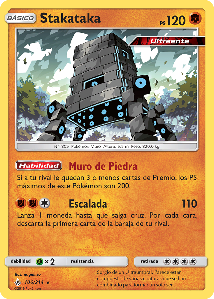
Using the following card in a game:

What is the probability of discarding 4 of your opponent’s cards?
- In a certain store, the probability of selling a device with a factory defect is 2%. What is the probability that the tenth device sold is the third with factory defects?